bachelor_thesis/prog/python/qqgg/analytical_xs.org

Investigaton of Monte-Carlo Methods

• Init
  • Required Modules
  • Utilities
• Implementation
  • Center of Mass Frame
• Calculations
  • Analytical Integration
  • Numerical Integration
    • Integral over θ
    • Integration over η
    • Using VEGAS
    • Testing the Statistics
  • Sampling and Analysis
    • Sampling the cosθ cross section
    • Observables
    • Sampling the η cross section
    • Sampling with VEGAS
    • Some Histograms with Rivet
      • Init
      • Plot the Histos

Init

Required Modules

  import numpy as np
  import matplotlib.pyplot as plt
  import monte_carlo

Utilities

%run ../utility.py
%load_ext autoreload
%aimport monte_carlo
%autoreload 1

The autoreload extension is already loaded. To reload it, use:
  %reload_ext autoreload

Implementation

Center of Mass Frame

  """
  Implementation of the analytical cross section for q q_bar ->
  gamma gamma

  Author: Valentin Boettcher <hiro@protagon.space>
  """

  import numpy as np

  # NOTE: a more elegant solution would be a decorator
  def energy_factor(charge, esp):
      """
      Calculates the factor common to all other values in this module

      Arguments:
      esp -- center of momentum energy in GeV
      charge -- charge of the particle in units of the elementary charge
      """

      return charge ** 4 / (137.036 * esp) ** 2 / 6


  def diff_xs(θ, charge, esp):
      """
      Calculates the differential cross section as a function of the
      azimuth angle θ in units of 1/GeV².

      Here dΩ=sinθdθdφ

      Arguments:
      θ -- azimuth angle
      esp -- center of momentum energy in GeV
      charge -- charge of the particle in units of the elementary charge
      """

      f = energy_factor(charge, esp)
      return f * ((np.cos(θ) ** 2 + 1) / np.sin(θ) ** 2)


  def diff_xs_cosθ(cosθ, charge, esp):
      """
      Calculates the differential cross section as a function of the
      cosine of the azimuth angle θ in units of 1/GeV².

      Here dΩ=d(cosθ)dφ

      Arguments:
      cosθ -- cosine of the azimuth angle
      esp -- center of momentum energy in GeV
      charge -- charge of the particle in units of the elementary charge
      """

      f = energy_factor(charge, esp)
      return f * ((cosθ ** 2 + 1) / (1 - cosθ ** 2))


  def diff_xs_eta(η, charge, esp):
      """
      Calculates the differential cross section as a function of the
      pseudo rapidity of the photons in units of 1/GeV^2.

      This is actually the crossection dσ/(dφdη).

      Arguments:
      η -- pseudo rapidity
      esp -- center of momentum energy in GeV
      charge -- charge of the particle in units of the elementary charge
      """

      f = energy_factor(charge, esp)
      return f * (np.tanh(η) ** 2 + 1)


  def diff_xs_p_t(p_t, charge, esp):
      """
      Calculates the differential cross section as a function of the
      transverse momentum (p_t) of the photons in units of 1/GeV^2.

      This is actually the crossection dσ/(dφdp_t).

      Arguments:
      p_t -- transverse momentum in GeV
      esp -- center of momentum energy in GeV
      charge -- charge of the particle in units of the elementary charge
      """

      f = energy_factor(charge, esp)
      sqrt_fact = np.sqrt(1 - (2 * p_t / esp) ** 2)
      return f / p_t * (1 / sqrt_fact + sqrt_fact)


  def total_xs_eta(η, charge, esp):
      """
      Calculates the total cross section as a function of the pseudo
      rapidity of the photons in units of 1/GeV^2.  If the rapditiy is
      specified as a tuple, it is interpreted as an interval.  Otherwise
      the interval [-η, η] will be used.

      Arguments:
      η -- pseudo rapidity (tuple or number)
      esp -- center of momentum energy in GeV
      charge -- charge of the particle in units of the elementar charge
      """

      f = energy_factor(charge, esp)
      if not isinstance(η, tuple):
          η = (-η, η)

      if len(η) != 2:
          raise ValueError("Invalid η cut.")

      def F(x):
          return np.tanh(x) - 2 * x

      return 2 * np.pi * f * (F(η[0]) - F(η[1]))

Analytical Integration

And now calculate the cross section in picobarn.

  xs_gev = total_xs_eta(η, charge, esp)
  xs_pb = gev_to_pb(xs_gev)
  tex_value(xs_pb, unit=r'\pico\barn', prefix=r'\sigma = ',
            prec=6, save=('results', 'xs.tex'))

\(\sigma = \SI{0.053793}{\pico\barn}\)

Lets plot the total xs as a function of η.

  fig, ax = set_up_plot()
  η_s = np.linspace(0, 3, 1000)
  ax.plot(η_s, gev_to_pb(total_xs_eta(η_s, charge, esp)))
  ax.set_xlabel(r'$\eta$')
  ax.set_ylabel(r'$\sigma$ [pb]')
  ax.set_xlim([0, max(η_s)])
  ax.set_ylim(0)
  save_fig(fig, 'total_xs', 'xs', size=[2.5, 2.5])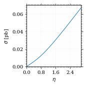

Compared to sherpa, it's pretty close.

  sherpa = 0.05380
  xs_pb - sherpa

-6.7112594623469635e-06

I had to set the runcard option EW_SCHEME: alpha0 to use the pure QED coupling constant.

Numerical Integration

Plot our nice distribution:

  plot_points = np.linspace(*plot_interval, 1000)

  fig, ax = set_up_plot()
  ax.plot(plot_points, gev_to_pb(diff_xs(plot_points, charge=charge, esp=esp)))
  ax.set_xlabel(r'$\theta$')
  ax.set_ylabel(r'$d\sigma/d\Omega$ [pb]')
  ax.set_xlim([plot_points.min(), plot_points.max()])
  ax.axvline(interval[0], color='gray', linestyle='--')
  ax.axvline(interval[1], color='gray', linestyle='--', label=rf'$|\eta|={η}$')
  ax.legend()
  save_fig(fig, 'diff_xs', 'xs', size=[2.5, 2.5])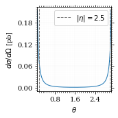

Define the integrand.

  def xs_pb_int(θ):
      return 2*np.pi*gev_to_pb(np.sin(θ)*diff_xs(θ, charge=charge, esp=esp))

  def xs_pb_int_η(η):
      return 2*np.pi*gev_to_pb(diff_xs_eta(η, charge, esp))

Plot the integrand. # TODO: remove duplication

  fig, ax = set_up_plot()
  ax.plot(plot_points, xs_pb_int(plot_points))
  ax.set_xlabel(r'$\theta$')
  ax.set_ylabel(r'$2\pi\cdot d\sigma/d\theta [pb]')
  ax.set_xlim([plot_points.min(), plot_points.max()])
  ax.axvline(interval[0], color='gray', linestyle='--')
  ax.axvline(interval[1], color='gray', linestyle='--', label=rf'$|\eta|={η}$')
  save_fig(fig, 'xs_integrand', 'xs', size=[3, 2.2])

Integral over θ

Intergrate σ with the mc method.

  xs_pb_res = monte_carlo.integrate(xs_pb_int, interval, epsilon=1e-3)
  xs_pb_res

IntegrationResult(result=0.05380076774689264, sigma=0.0009156046547219115, N=2383)

We gonna export that as tex.

  tex_value(*xs_pb_res.combined_result, unit=r'\pico\barn',
            prefix=r'\sigma = ', save=('results', 'xs_mc.tex'))
  tex_value(xs_pb_res.N, prefix=r'N = ', save=('results', 'xs_mc_N.tex'))

\(N = 2383\)

Integration over η

Plot the intgrand of the pseudo rap.

  fig, ax = set_up_plot()
  points = np.linspace(-4, 4, 1000)
  ax.set_xlim([-4, 4])
  ax.plot(points, xs_pb_int_η(points))
  ax.set_xlabel(r'$\eta$')
  ax.set_ylabel(r'$2\pi\cdot d\sigma/d\eta$ [pb]')
  ax.axvline(interval_η[0], color='gray', linestyle='--')
  ax.axvline(interval_η[1], color='gray', linestyle='--', label=rf'$|\eta|={η}$')
  save_fig(fig, 'xs_integrand_eta', 'xs', size=[3, 2])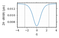

  xs_pb_η = monte_carlo.integrate(xs_pb_int_η,
                                  interval_η, epsilon=1e-3)
  xs_pb_η

IntegrationResult(result=0.053381188045107726, sigma=0.0009626020740618223, N=137)

As we see, the result is a little better if we use pseudo rapidity, because the differential cross section does not difverge anymore. But becase our η interval is covering the range where all the variance is occuring, the improvement is rather marginal.

And yet again export that as tex.

  tex_value(*xs_pb_η.combined_result, unit=r'\pico\barn', prefix=r'\sigma = ',
            save=('results', 'xs_mc_eta.tex'))
  tex_value(xs_pb_η.N, prefix=r'N = ', save=('results', 'xs_mc_eta_N.tex'))

\(N = 137\)

Using VEGAS

Now we use VEGAS on the θ parametrisation and see what happens.

  num_increments = 11
  xs_pb_vegas = monte_carlo.integrate_vegas(
      xs_pb_int,
      interval,
      num_increments=num_increments,
      alpha=1,
      increment_epsilon=0.001,
      acumulate=False,
  )
  xs_pb_vegas

VegasIntegrationResult(result=0.05353797358506919, sigma=0.00013283395611126086, N=2805, increment_borders=array([0.16380276, 0.2374099 , 0.34568281, 0.5094011 , 0.76958263,
       1.23235422, 1.91714873, 2.37499285, 2.63412137, 2.79640826,
       2.90423418, 2.9777899 ]), vegas_iterations=9500)

This is pretty good, although the variance reduction may be achieved partially by accumulating the results from all runns. Here this gives us one order of magnitude more than we wanted.

And export that as tex.

  tex_value(*xs_pb_vegas.combined_result, unit=r'\pico\barn',
            prefix=r'\sigma = ', save=('results', 'xs_mc_θ_vegas.tex'))
  tex_value(xs_pb_vegas.N, prefix=r'N = ', save=('results', 'xs_mc_θ_vegas_N.tex'))
  tex_value(num_increments, prefix=r'K = ', save=('results', 'xs_mc_θ_vegas_K.tex'))

\(K = 11\)

Surprisingly, acumulation, the result ain't much different. This depends, of course, on the iteration count.

  monte_carlo.integrate_vegas(
      xs_pb_int,
      interval,
      num_increments=num_increments,
      alpha=1,
      increment_epsilon=0.001,
      acumulate=True,
  )

VegasIntegrationResult(result=0.053785157752621354, sigma=1.887850854134335e-05, N=2805, increment_borders=array([0.16380276, 0.23716945, 0.34540806, 0.50930035, 0.76937514,
       1.22945366, 1.91539567, 2.37452676, 2.63392477, 2.79705411,
       2.9048259 , 2.9777899 ]), vegas_iterations=2563)

Let's define some little helpers.

  """
  Some shorthands for common plotting tasks related to the investigation
  of monte-carlo methods in one rimension.

  Author: Valentin Boettcher <hiro at protagon.space>
  """

  import matplotlib.pyplot as plt
  import matplotlib.gridspec as gridspec
  import yoda as yo
  from collections.abc import Iterable
  import yoda.plotting as yplt
  import numpy as np
  from utility import *


  def plot_increments(ax, increment_borders, label=None, *args, **kwargs):
      """Plot the increment borders from a list.  The first and last one

      :param ax: the axis on which to draw
      :param list increment_borders: the borders of the increments
      :param str label: the label to apply to one of the vertical lines
      """

      ax.axvline(x=increment_borders[1], label=label, *args, **kwargs)

      for increment in increment_borders[1:-1]:
          ax.axvline(x=increment, *args, **kwargs)


  def plot_vegas_weighted_distribution(
      ax, points, dist, increment_borders, *args, **kwargs
  ):
      """Plot the distribution with VEGAS weights applied.

      :param ax: axis
      :param points: points
      :param dist: distribution
      :param increment_borders: increment borders
      """

      num_increments = increment_borders.size
      weighted_dist = dist.copy()

      for left_border, right_border in zip(increment_borders[:-1], increment_borders[1:]):
          length = right_border - left_border
          mask = (left_border <= points) & (points <= right_border)
          weighted_dist[mask] = dist[mask] * num_increments * length

      ax.plot(points, weighted_dist, *args, **kwargs)


  def plot_stratified_rho(ax, points, increment_borders, *args, **kwargs):
      """Plot the weighting distribution resulting from the increment
      borders.

      :param ax: axis
      :param points: points
      :param increment_borders: increment borders

      """

      num_increments = increment_borders.size
      ρ = np.empty_like(points)
      for left_border, right_border in zip(increment_borders[:-1], increment_borders[1:]):
          length = right_border - left_border
          mask = (left_border <= points) & (points <= right_border)
          ρ[mask] = 1 / (num_increments * length)

      ax.plot(points, ρ, *args, **kwargs)

And now we plot the integrand with the incremens.

  fig, ax = set_up_plot()
  ax.set_xlim(*interval)
  ax.set_xlabel(r"$\theta$")
  ax.set_ylabel(r"$2\pi\cdot d\sigma/d\theta$ [pb]")
  ax.set_ylim([0, 0.09])

  ax.plot(plot_points, xs_pb_int(plot_points), label="Distribution")

  plot_increments(
      ax,
      xs_pb_vegas.increment_borders,
      label="Increment Borders",
      color="gray",
      linestyle="--",
  )

  plot_vegas_weighted_distribution(
      ax,
      plot_points,
      xs_pb_int(plot_points),
      xs_pb_vegas.increment_borders,
      label="Weighted Distribution",
  )

  ax.legend(fontsize="small", loc="lower left")
  save_fig(fig, "xs_integrand_vegas", "xs", size=[5, 3])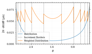

Testing the Statistics

Let's battle test the statistics.

  num_runs = 1000
  num_within = 0

  for _ in range(num_runs):
      val, err = \
          monte_carlo.integrate(xs_pb_int, interval, epsilon=1e-3).combined_result
      if abs(xs_pb - val) <= err:
          num_within += 1

  num_within/num_runs

0.691

So we see: the standard deviation is sound.

Doing the same thing with VEGAS works as well.

  num_runs = 1000
  num_within = 0
  for _ in range(num_runs):
      val, err = \
          monte_carlo.integrate_vegas(xs_pb_int, interval,
                                      num_increments=10, alpha=1,
                                      epsilon=1e-3, acumulate=False,
                                      vegas_point_density=100).combined_result

      if abs(xs_pb - val) <= err:
          num_within += 1
  num_within/num_runs

0.686

Sampling and Analysis

Define the sample number.

  sample_num = 1_000_000
  tex_value(
      sample_num, prefix="N = ", save=("results", "4imp-sample-size.tex"),
  )

\(N = 1000000\)

Let's define shortcuts for our distributions. The 2π are just there for formal correctnes. Factors do not influecence the outcome.

  def dist_cosθ(x):
      return gev_to_pb(diff_xs_cosθ(x, charge, esp))

  def dist_η(x):
      return gev_to_pb(diff_xs_eta(x, charge, esp))

Sampling the cosθ cross section

Now we monte-carlo sample our distribution. We observe that the efficiency his very bad!

  cosθ_sample, cosθ_efficiency = \
      monte_carlo.sample_unweighted_array(sample_num, dist_cosθ,
                                          interval_cosθ, report_efficiency=True,
                                          cache='cache/bare_cos_theta',
                                          proc='auto')
  cosθ_efficiency

0.02744127583441648

Let's save that.

  tex_value(
      cosθ_efficiency * 100,
      prefix=r"\mathfrak{e} = ",
      suffix=r"\%",
      save=("results", "naive_th_samp.tex"),
  )

\(\mathfrak{e} = 3\%\)

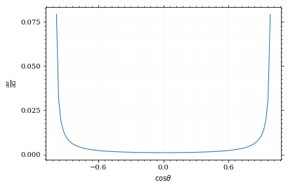
Our distribution has a lot of variance, as can be seen by plotting it.

  pts = np.linspace(*interval_cosθ, 100)
  fig, ax = set_up_plot()
  ax.plot(pts, dist_cosθ(pts))
  ax.set_xlabel(r'$\cos\theta$')
  ax.set_ylabel(r'$\frac{d\sigma}{d\Omega}$')

Text(0, 0.5, '$\\frac{d\\sigma}{d\\Omega}$')

We define a friendly and easy to integrate upper limit function.

  fig, ax = set_up_plot()
  upper_limit = dist_cosθ(interval_cosθ[0]) / interval_cosθ[0] ** 2
  upper_base = dist_cosθ(0)


  def upper(x):
      return upper_base + upper_limit * x ** 2


  def upper_int(x):
      return upper_base * x + upper_limit * x ** 3 / 3


  ax.plot(pts, upper(pts), label="upper bound")
  ax.plot(pts, dist_cosθ(pts), label=r"$f_{\cos\theta}$")

  ax.legend(fontsize='small')
  ax.set_xlabel(r"$\cos\theta$")
  ax.set_ylabel(r"$\frac{d\sigma}{d\cos\theta}$ [pb]")
  save_fig(fig, "upper_bound", "xs_sampling", size=(3, 2.5))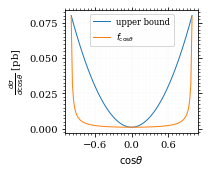

To increase our efficiency, we have to specify an upper bound. That is at least a little bit better. The numeric inversion is horribly inefficent.

  cosθ_sample_tuned, cosθ_efficiency_tuned = monte_carlo.sample_unweighted_array(
      sample_num,
      dist_cosθ,
      interval_cosθ,
      report_efficiency=True,
      proc="auto",
      cache="cache/bare_cos_theta_tuned",
      upper_bound=[upper, upper_int],
  )
  cosθ_efficiency_tuned

0.07903728511692736

<<cosθ-bare-eff>>

  tex_value(
      cosθ_efficiency_tuned * 100,
      prefix=r"\mathfrak{e} = ",
      suffix=r"\%",
      save=("results", "tuned_th_samp.tex"),
  )

\(\mathfrak{e} = 8\%\)

Nice! And now draw some histograms.

We define an auxilliary method for convenience.

  def draw_histogram(
      ax,
      histogram,
      errorbars=True,
      hist_kwargs=dict(color="#1f77b4"),
      errorbar_kwargs=dict(color="orange"),
      normalize_to=None,
  ):
      """Draws a histogram with optional errorbars using the step style.

      :param ax: axis to draw on
      :param histogram: an array of the form [heights, edges]
      :param hist_kwargs: keyword args to pass to `ax.step`
      :param errorbar_kwargs: keyword args to pass to `ax.errorbar`
      :param normalize_to: if set, the histogram will be normalized to the value
      :returns: the given axis
      """

      heights, edges = histogram
      centers = (edges[1:] + edges[:-1]) / 2
      deviations = (
          (errorbars if isinstance(errorbars, (np.ndarray, list)) else np.sqrt(heights))
          if errorbars is not False
          else None
      )

      if normalize_to is not None:
          integral = hist_integral(histogram)
          heights = heights / integral * normalize_to
          if errorbars is not False:
              deviations = deviations / integral * normalize_to

      if errorbars is not False:
          ax.errorbar(centers, heights, deviations, linestyle="none", **errorbar_kwargs)

      ax.step(edges, [heights[0], *heights], **hist_kwargs)
      ax.set_xlim(*[edges[0], edges[-1]])

      return ax


  @functools.wraps(yplt.plot)
  def yoda_plot_wrapper(*args, **kwargs):
      fig, axs = yplt.plot(*args, **kwargs)
      if isinstance(axs, Iterable):
          axs = [set_up_axis(ax) for ax in axs if ax is not None]
      else:
          axs = set_up_axis(axs)

      return fig, axs

  def samples_to_yoda(samples, bins, range=None, **kwargs):
      if range is None:
          range = [min(samples), max(samples)]

      hist = yo.Histo1D(bins, *range, **kwargs)
      for sample in samples:
          hist.fill(sample)

      return hist

  def draw_histo_auto(
      points, xlabel, title="", bins=50, range=None, rethist=False, **kwargs
  ):
      """Creates a histogram figure from sample points, normalized to unity.

      :param points: samples
      :param xlabel: label of the x axis
      :param bins: number of bins
      :param range: the range of the values
      :param rethist: whether to return the histogram as third argument
      :returns: figure, axis
      """

      hist = yo.Histo1D(
          bins, *(range if range is not None else [min(points), max(points)]), title
      )

      for point in points:
          hist.fill(point)

      plot = yoda_plot_wrapper(hist, xlabel=xlabel, **kwargs)
      return (*plot, hist) if rethist else plot

The histogram for cosθ.

  from importlib import reload

  reload(yplt)
  fig, _, hist_cosθ = draw_histo_auto(
      cosθ_sample,
      r"$\cos\theta$",
      title=r"own implementation",
      rethist=True,
      range=interval_cosθ,
  )
  save_fig(fig, "histo_cos_theta", "xs", size=(4, 3))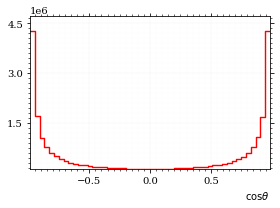

Observables

Now we define some utilities to draw real 4-momentum samples.

  @numpy_cache("momentum_cache")
  def sample_momenta(sample_num, interval, charge, esp, seed=None, **kwargs):
      """Samples `sample_num` unweighted photon 4-momenta from the
      cross-section. Superflous kwargs are passed on to
      `sample_unweighted_array`.

      :param sample_num: number of samples to take
      :param interval: cosθ interval to sample from
      :param charge: the charge of the quark
      :param esp: center of mass energy
      :param seed: the seed for the rng, optional, default is system
          time

      :returns: an array of 4 photon momenta

      :rtype: np.ndarray

      """

      cosθ_sample = monte_carlo.sample_unweighted_array(
          sample_num, lambda x: diff_xs_cosθ(x, charge, esp), interval_cosθ, **kwargs
      )
      φ_sample = np.random.uniform(0, 1, sample_num)

      def make_momentum(esp, cosθ, φ):
          sinθ = np.sqrt(1 - cosθ ** 2)
          return np.array([1, sinθ * np.cos(φ), sinθ * np.sin(φ), cosθ],) * esp / 2

      momenta = np.array(
          [make_momentum(esp, cosθ, φ) for cosθ, φ in np.array([cosθ_sample, φ_sample]).T]
      )
      return momenta

To generate histograms of other obeservables, we have to define them as functions on 4-impuleses. Using those to transform samples is analogous to transforming the distribution itself.

  """This module defines some observables on arrays of 4-pulses."""
  import numpy as np

  def p_t(p):
      """Transverse momentum

      :param p: array of 4-momenta
      """

      return np.linalg.norm(p[:,1:3], axis=1)

  def η(p):
      """Pseudo rapidity.

      :param p: array of 4-momenta
      """

      return np.arccosh(np.linalg.norm(p[:,1:], axis=1)/p_t(p))*np.sign(p[:, 3])

And import them.

  %aimport tangled.observables
  obs = tangled.observables

Lets try it out.

  momentum_sample = sample_momenta(
      sample_num,
      interval_cosθ,
      charge,
      esp,
      cache="cache/bare_cos_theta",
      proc=3,
      momentum_cache="cache/momenta_bare_cos_theta",
  )
  momentum_sample

Trying cache
array([[100.        ,  54.98191622,  34.53483728, -76.05480855],
       [100.        ,  87.95719691,  30.53342542, -36.48618154],
       [100.        ,  29.02952127,  15.22393108, -94.47496397],
       ...,
       [100.        ,  37.62519445,  37.66247038, -84.65153907],
       [100.        ,  75.22515369,   0.79738586,  65.88277793],
       [100.        ,  26.58309333,   4.84203005, -96.28028819]])

Now let's make a histogram of the η distribution.

  η_sample = obs.η(momentum_sample)
  fig, ax, hist_obs_η = draw_histo_auto(
      η_sample, r"$\eta$", title="own implementation", range=interval_η, rethist=True
  )
  hist_obs_η.normalize(1)
  save_fig(fig, "histo_eta", "xs_sampling", size=[3, 3])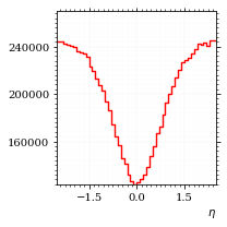

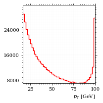
And the same for the p_t (transverse momentum) distribution.

  p_t_sample = obs.p_t(momentum_sample)
  fig, ax, hist_obs_pt = draw_histo_auto(
      p_t_sample,
      r"$p_T$ [GeV]",
      title="own implementation",
      range=interval_pt,
      rethist=True,
  )
  save_fig(fig, "histo_pt", "xs_sampling", size=[3, 3])

  BrokenPipeErrorTraceback (most recent call last)
  <ipython-input-202-d07958ed2945> in <module>
        7     rethist=True,
        8 )
  ----> 9 save_fig(fig, "histo_pt", "xs_sampling", size=[3, 3])

  ~/Documents/Projects/UNI/Bachelor/prog/python/qqgg/utility.py in save_fig(fig, title, folder, size)
      189
      190     fig.savefig(f"./figs/{folder}/{title}.pdf")
  --> 191     fig.savefig(f"./figs/{folder}/{title}.pgf")
      192
      193

  /usr/lib/python3.8/site-packages/matplotlib/figure.py in savefig(self, fname, transparent, **kwargs)
     2201             self.patch.set_visible(frameon)
     2202
  -> 2203         self.canvas.print_figure(fname, **kwargs)
     2204
     2205         if frameon:

  /usr/lib/python3.8/site-packages/matplotlib/backend_bases.py in print_figure(self, filename, dpi, facecolor, edgecolor, orientation, format, bbox_inches, **kwargs)
     2096
     2097             try:
  -> 2098                 result = print_method(
     2099                     filename,
     2100                     dpi=dpi,

  /usr/lib/python3.8/site-packages/matplotlib/backends/backend_pgf.py in print_pgf(self, fname_or_fh, *args, **kwargs)
      888             if not cbook.file_requires_unicode(file):
      889                 file = codecs.getwriter("utf-8")(file)
  --> 890             self._print_pgf_to_fh(file, *args, **kwargs)
      891
      892     def _print_pdf_to_fh(self, fh, *args, **kwargs):

  /usr/lib/python3.8/site-packages/matplotlib/cbook/deprecation.py in wrapper(*args, **kwargs)
      356                 f"%(removal)s.  If any parameter follows {name!r}, they "
      357                 f"should be pass as keyword, not positionally.")
  --> 358         return func(*args, **kwargs)
      359
      360     return wrapper

  /usr/lib/python3.8/site-packages/matplotlib/backends/backend_pgf.py in _print_pgf_to_fh(self, fh, dryrun, bbox_inches_restore, *args, **kwargs)
      870                                      RendererPgf(self.figure, fh),
      871                                      bbox_inches_restore=bbox_inches_restore)
  --> 872         self.figure.draw(renderer)
      873
      874         # end the pgfpicture environment

  /usr/lib/python3.8/site-packages/matplotlib/artist.py in draw_wrapper(artist, renderer, *args, **kwargs)
       36                 renderer.start_filter()
       37
  ---> 38             return draw(artist, renderer, *args, **kwargs)
       39         finally:
       40             if artist.get_agg_filter() is not None:

  /usr/lib/python3.8/site-packages/matplotlib/figure.py in draw(self, renderer)
     1733
     1734             self.patch.draw(renderer)
  -> 1735             mimage._draw_list_compositing_images(
     1736                 renderer, self, artists, self.suppressComposite)
     1737

  /usr/lib/python3.8/site-packages/matplotlib/image.py in _draw_list_compositing_images(renderer, parent, artists, suppress_composite)
      135     if not_composite or not has_images:
      136         for a in artists:
  --> 137             a.draw(renderer)
      138     else:
      139         # Composite any adjacent images together

  /usr/lib/python3.8/site-packages/matplotlib/artist.py in draw_wrapper(artist, renderer, *args, **kwargs)
       36                 renderer.start_filter()
       37
  ---> 38             return draw(artist, renderer, *args, **kwargs)
       39         finally:
       40             if artist.get_agg_filter() is not None:

  /usr/lib/python3.8/site-packages/matplotlib/axes/_base.py in draw(self, renderer, inframe)
     2628             renderer.stop_rasterizing()
     2629
  -> 2630         mimage._draw_list_compositing_images(renderer, self, artists)
     2631
     2632         renderer.close_group('axes')

  /usr/lib/python3.8/site-packages/matplotlib/image.py in _draw_list_compositing_images(renderer, parent, artists, suppress_composite)
      135     if not_composite or not has_images:
      136         for a in artists:
  --> 137             a.draw(renderer)
      138     else:
      139         # Composite any adjacent images together

  /usr/lib/python3.8/site-packages/matplotlib/artist.py in draw_wrapper(artist, renderer, *args, **kwargs)
       36                 renderer.start_filter()
       37
  ---> 38             return draw(artist, renderer, *args, **kwargs)
       39         finally:
       40             if artist.get_agg_filter() is not None:

  /usr/lib/python3.8/site-packages/matplotlib/axis.py in draw(self, renderer, *args, **kwargs)
     1239         self._update_label_position(renderer)
     1240
  -> 1241         self.label.draw(renderer)
     1242
     1243         self._update_offset_text_position(ticklabelBoxes, ticklabelBoxes2)

  /usr/lib/python3.8/site-packages/matplotlib/artist.py in draw_wrapper(artist, renderer, *args, **kwargs)
       36                 renderer.start_filter()
       37
  ---> 38             return draw(artist, renderer, *args, **kwargs)
       39         finally:
       40             if artist.get_agg_filter() is not None:

  /usr/lib/python3.8/site-packages/matplotlib/text.py in draw(self, renderer)
      683
      684         with _wrap_text(self) as textobj:
  --> 685             bbox, info, descent = textobj._get_layout(renderer)
      686             trans = textobj.get_transform()
      687

  /usr/lib/python3.8/site-packages/matplotlib/text.py in _get_layout(self, renderer)
      297             clean_line, ismath = self._preprocess_math(line)
      298             if clean_line:
  --> 299                 w, h, d = renderer.get_text_width_height_descent(
      300                     clean_line, self._fontproperties, ismath=ismath)
      301             else:

  /usr/lib/python3.8/site-packages/matplotlib/backends/backend_pgf.py in get_text_width_height_descent(self, s, prop, ismath)
      755
      756         # get text metrics in units of latex pt, convert to display units
  --> 757         w, h, d = (LatexManager._get_cached_or_new()
      758                    .get_width_height_descent(s, prop))
      759         # TODO: this should be latex_pt_to_in instead of mpl_pt_to_in

  /usr/lib/python3.8/site-packages/matplotlib/backends/backend_pgf.py in get_width_height_descent(self, text, prop)
      356
      357         # send textbox to LaTeX and wait for prompt
  --> 358         self._stdin_writeln(textbox)
      359         try:
      360             self._expect_prompt()

  /usr/lib/python3.8/site-packages/matplotlib/backends/backend_pgf.py in _stdin_writeln(self, s)
      257         self.latex_stdin_utf8.write(s)
      258         self.latex_stdin_utf8.write("\n")
  --> 259         self.latex_stdin_utf8.flush()
      260
      261     def _expect(self, s):

  BrokenPipeError: [Errno 32] Broken pipe

That looks somewhat fishy, but it isn't.

  fig, ax = set_up_plot()
  points = np.linspace(interval_pt[0], interval_pt[1] - .01, 1000)
  ax.plot(points, gev_to_pb(diff_xs_p_t(points, charge, esp)))
  ax.set_xlabel(r'$p_T$')
  ax.set_xlim(interval_pt[0], interval_pt[1] + 1)
  ax.set_ylim([0, gev_to_pb(diff_xs_p_t(interval_pt[1] -.01, charge, esp))])
  ax.set_ylabel(r'$\frac{d\sigma}{dp_t}$ [pb]')
  save_fig(fig, 'diff_xs_p_t', 'xs_sampling', size=[4, 2])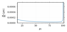

this is strongly peaked at p_t=100GeV. (The jacobian goes like 1/x there!)

Sampling the η cross section

An again we see that the efficiency is way, way! better…

  η_sample, η_efficiency = monte_carlo.sample_unweighted_array(
      1000,
      dist_η,
      interval_η,
      report_efficiency=True,
      proc="auto",
      #cache="cache/sample_bare_eta",
  )
  tex_value(
      η_efficiency * 100,
      prefix=r"\mathfrak{e} = ",
      suffix=r"\%",
      save=("results", "eta_eff.tex"),
  )

\(\mathfrak{e} = 41\%\)

<<η-eff>>

Let's draw a histogram to compare with the previous results.

  η_hist = samples_to_yoda(η_sample, 50, title="sampled from $d\sigma / d\eta$")
  reload(yplt)
  η_hist.normalize(1)
  η_hist.setAnnotation('ratioref', True)

  yoda_plot_wrapper([hist_obs_η, η_hist], errorbars=True)
  # fig, (ax_hist, ax_ratio) = draw_ratio_plot(
  #     [
  #         dict(hist=η_hist, hist_kwargs=dict(label=r"sampled from $d\sigma / d\eta$"),),
  #         dict(
  #             hist=hist_obs_η,
  #             hist_kwargs=dict(
  #                 label=r"sampled from $d\sigma / d\cos\theta$", color="black"
  #             ),
  #         ),
  #     ],
  # )

  # ax_hist.legend(loc="upper center", fontsize="small")
  # ax_ratio.set_xlabel(r"$\eta$")
  #save_fig(fig, "comparison_eta", "xs_sampling", size=(4, 4))

<Figure

size

576x432

with

2

Axes>

(<matplotlib.axes._subplots.AxesSubplot at 0x7f923b1ea070> <matplotlib.axes._subplots.AxesSubplot at 0x7f923b18bdc0>)

Looks good to me :).

Sampling with VEGAS

To get the increments, we have to let VEGAS loose on our distribution. We throw away the integral, but keep the increments.

  K = 10
  increments = monte_carlo.integrate_vegas(
      dist_cosθ, interval_cosθ, num_increments=K, alpha=1, increment_epsilon=0.001
  ).increment_borders
  tex_value(
      K, prefix=r"K = ", save=("results", "vegas_samp_num_increments.tex"),
  )
  increments

array([-0.9866143 , -0.96980073, -0.93072072, -0.83891589, -0.6017223 ,
        0.00829172,  0.6071626 ,  0.83981042,  0.93107467,  0.96951636,
        0.9866143 ])

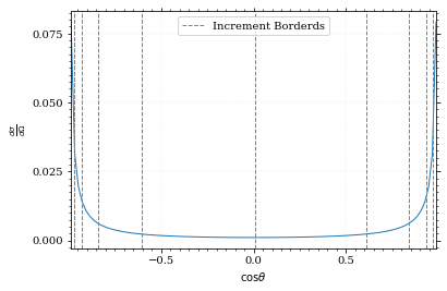
Visualizing the increment borders gives us the information we want.

  pts = np.linspace(*interval_cosθ, 100)
  fig, ax = set_up_plot()
  ax.plot(pts, dist_cosθ(pts))
  ax.set_xlabel(r'$\cos\theta$')
  ax.set_ylabel(r'$\frac{d\sigma}{d\Omega}$')
  ax.set_xlim(*interval_cosθ)
  plot_increments(ax, increments,
                  label='Increment Borderds', color='gray', linestyle='--')
  ax.legend()

<matplotlib.legend.Legend at 0x7f924d64e730>

We can now plot the reweighted distribution to observe the variance reduction visually.

  pts = np.linspace(*interval_cosθ, 1000)
  fig, ax = set_up_plot()
  ax.plot(pts, dist_cosθ(pts), label="Distribution")
  plot_vegas_weighted_distribution(
      ax, pts, dist_cosθ(pts), increments, label="Weighted Distribution"
  )
  ax.set_xlabel(r"$\cos\theta$")
  ax.set_ylabel(r"$\frac{d\sigma}{d\cos\theta}$")
  ax.set_xlim(*interval_cosθ)
  plot_increments(
      ax, increments, label="Increment Borderds", color="gray", linestyle="--"
  )
  ax.legend(fontsize="small")
  save_fig(fig, "vegas_strat_dist", "xs_sampling", size=(3, 2.3))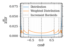

I am batman! Let's plot the weighting distribution.

  pts = np.linspace(*interval_cosθ, 1000)
  fig, ax = set_up_plot()
  plot_stratified_rho(ax, pts, increments)
  ax.set_xlabel(r"$\cos\theta$")
  ax.set_ylabel(r"$\rho")
  ax.set_xlim(*interval_cosθ)
  save_fig(fig, "vegas_rho", "xs_sampling", size=(3, 2.3))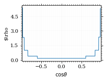

Now, draw a sample and look at the efficiency.

  cosθ_sample_strat, cosθ_efficiency_strat = monte_carlo.sample_unweighted_array(
      sample_num,
      dist_cosθ,
      increment_borders=increments,
      report_efficiency=True,
      proc="auto",
      cache="cache/sample_bare_cos_theta_vegas",
  )
  cosθ_efficiency_strat

0.5954571428571428

  tex_value(
      cosθ_efficiency_strat * 100,
      prefix=r"\mathfrak{e} = ",
      suffix=r"\%",
      save=("results", "strat_th_samp.tex"),
  )

\(\mathfrak{e} = 60\%\)

If we compare that to /hiro/bachelor_thesis/src/commit/f157b525328f012d5d5ea1acc6820047e5af6f55/prog/python/qqgg/cos%CE%B8-bare-eff, we can see the improvement :P. It is even better the /hiro/bachelor_thesis/src/commit/f157b525328f012d5d5ea1acc6820047e5af6f55/prog/python/qqgg/%CE%B7-eff. The histogram looks just the same.

fig, _ = draw_histo_auto(cosθ_sample_strat, r'$\cos\theta$')
save_fig(fig, 'histo_cos_theta_strat', 'xs', size=(4,3))

  TypeErrorTraceback (most recent call last)
  <ipython-input-148-ff4d6a24ae42> in <module>
  ----> 1 fig, _ = draw_histo_auto(cosθ_sample_strat, r'$\cos\theta$')
        2 save_fig(fig, 'histo_cos_theta_strat', 'xs', size=(4,3))

  <ipython-input-132-507ea080dcd6> in draw_histo_auto(points, xlabel, bins, range, rethist, **kwargs)
       70
       71
  ---> 72     return yoda_nplot_wrapper(hist, xlabel=xlabel, **kwargs)

  <ipython-input-132-507ea080dcd6> in yoda_nplot_wrapper(*args, **kwargs)
       42 @functools.wraps(yplt.nplot)
       43 def yoda_nplot_wrapper(*args, **kwargs):
  ---> 44     fig, axs = yplt.nplot(*args, **kwargs)
       45     if isinstance(axs, iterable):
       46         axs = [set_up_axis(ax) for ax in axs]

  /usr/lib/python3.8/site-packages/yoda/plotting.py in nplot(hs, outfiles, ratio, show, nproc, **plotkeys)
      446     else:
      447         ## Run this way in the 1 proc case for easier debugging
  --> 448         rtn = [_plot1arg(args) for args in argslist]
      449
      450     if show:

  /usr/lib/python3.8/site-packages/yoda/plotting.py in <listcomp>(.0)
      446     else:
      447         ## Run this way in the 1 proc case for easier debugging
  --> 448         rtn = [_plot1arg(args) for args in argslist]
      449
      450     if show:

  /usr/lib/python3.8/site-packages/yoda/plotting.py in _plot1arg(args)
      397 def _plot1arg(args):
      398     "Helper function for mplot, until Py >= 3.3 multiprocessing.pool.starmap() is available"
  --> 399     print(args)
      400     return plot(*args)
      401

  include/generated/Bin1D_Dbn1D.pyx in yoda.core.Bin1D_Dbn1D.__repr__()

  TypeError: must be real number, not builtin_function_or_method

Some Histograms with Rivet

Init

  import yoda

Plot the Histos

  def yoda_to_numpy(histo):
      histo.normalize(
          histo.numEntries() * ((histo.xMax() - histo.xMin()) / histo.numBins())
      )
      edges = np.append(histo.xMins(), histo.xMax())
      heights = histo.yVals().astype(int)

      return heights, edges


  def draw_yoda_histo_auto(h, xlabel, **kwargs):
      hist = yoda_to_numpy(h)
      fig, ax = set_up_plot()
      draw_histogram(ax, hist, errorbars=True, normalize_to=1, **kwargs)

      ax.set_xlabel(xlabel)
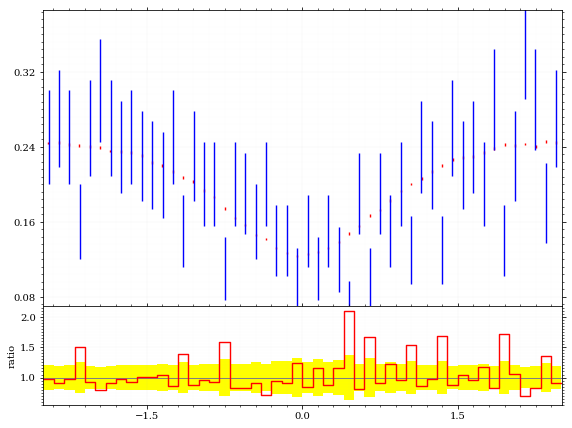
      return fig, ax

  yoda_file = yoda.read("../../runcards/qqgg/analysis/Analysis.yoda")
  sherpa_histos = {
      "pT": dict(reference=hist_obs_pt, label="$p_T$ [GeV]"),
      "eta": dict(reference=hist_obs_η, label=r"$\eta$"),
      "cos_theta": dict(reference=hist_cosθ, label=r"$\cos\theta$"),
  }

  for key, sherpa_hist in sherpa_histos.items():
      yoda_hist = yoda_to_numpy(yoda_file["/MC_DIPHOTON_SIMPLE/" + key])
      label = sherpa_hist["label"]
      fig, (ax_hist, ax_ratio) = draw_ratio_plot(
          [
              dict(
                  hist=yoda_hist,
                  hist_kwargs=dict(
                      label="Sherpa Reference"
                  ),
              ),
              dict(
                  hist=sherpa_hist["reference"],
                  hist_kwargs=dict(label="Own Implementation"),
              ),
          ],
      )
      ax_ratio.set_xlabel(label)
      save_fig(fig, "histo_sherpa_" + key, "xs_sampling", size=(4, 3.5))

NameErrorTraceback (most recent call last)
<ipython-input-151-c0fdcee231b0> in <module>
      1 yoda_file = yoda.read("../../runcards/qqgg/analysis/Analysis.yoda")
      2 sherpa_histos = {
----> 3     "pT": dict(reference=hist_obs_pt, label="$p_T$ [GeV]"),
      4     "eta": dict(reference=hist_obs_η, label=r"$\eta$"),
      5     "cos_theta": dict(reference=hist_cosθ, label=r"$\cos\theta$"),

NameError: name 'hist_obs_pt' is not defined

  %aimport yoda.plotting
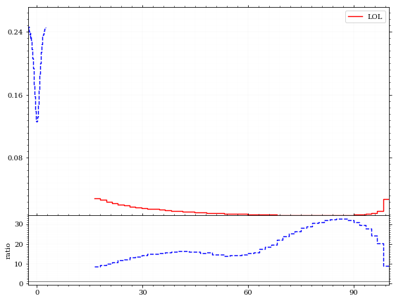
  hist = yoda_file["/MC_DIPHOTON_SIMPLE/pT"]
  hist.setAnnotation('ratioref', True)
  hist.setAnnotation('Title', "LOL")
  #hist.annotationsDict()
  fig, (ax_hist, ax_ratio) =yoda.plotting.plot([yoda_file["/MC_DIPHOTON_SIMPLE/pT"], yoda_file["/MC_DIPHOTON_SIMPLE/eta"]], ratio=True)
  set_up_axis(ax_hist)
  set_up_axis(ax_ratio)
  ax_hist.legend()

<matplotlib.legend.Legend at 0x7f924b270910>