bachelor_thesis/prog/python/qqgg/analytical_xs.org

• Init
  • Required Modules
  • Utilities
• Implementation
• Calculations
  • XS qq -> gamma gamma
    • Analytical Integratin
    • Numerical Integration
    • Sampling and Analysis

Init

Required Modules

  import numpy as np
  import matplotlib.pyplot as plt

Utilities

%run ../utility.py
%load_ext autoreload
%aimport monte_carlo

Implementation

  """
  Implementation of the analytical cross section for q q_bar ->
  gamma gamma

  Author: Valentin Boettcher <hiro@protagon.space>
  """

  import numpy as np
  from scipy.constants import alpha

  # NOTE: a more elegant solution would be a decorator
  def energy_factor(charge, esp):
      """
      Calculates the factor common to all other values in this module

      Arguments:
      esp -- center of momentum energy in GeV
      charge -- charge of the particle in units of the elementary charge
      """

      return charge**4*(alpha/esp)**2/6


  def diff_xs(θ, charge, esp):
      """
      Calculates the differential cross section as a function of the
      azimuth angle θ in units of 1/GeV².

      Arguments:
      θ -- azimuth angle
      esp -- center of momentum energy in GeV
      charge -- charge of the particle in units of the elementary charge
      """

      f = energy_factor(charge, esp)
      return f*((np.cos(θ)**2+1)/np.sin(θ)**2)

  def diff_xs_cosθ(cosθ, charge, esp):
      """
      Calculates the differential cross section as a function of the
      cosine of the azimuth angle θ in units of 1/GeV².

      Arguments:
      cosθ -- cosine of the azimuth angle
      esp -- center of momentum energy in GeV
      charge -- charge of the particle in units of the elementary charge
      """

      f = energy_factor(charge, esp)
      return f*((cosθ**2+1)/(1-cosθ**2))

  def diff_xs_eta(η, charge, esp):
      """
      Calculates the differential cross section as a function of the
      pseudo rapidity of the photons in units of 1/GeV^2.

      Arguments:
      η -- pseudo rapidity
      esp -- center of momentum energy in GeV
      charge -- charge of the particle in units of the elementary charge
      """

      f = energy_factor(charge, esp)
      return f*(2*np.cosh(η)**2 - 1)

  def diff_xs_pt(pt, charge, esp):
      """
      Calculates the differential cross section as a function of the
      transversal impulse of the photons in units of 1/GeV^2.

      Arguments:
      η -- transversal impulse
      esp -- center of momentum energy in GeV
      charge -- charge of the particle in units of the elementary charge
      """

      f = energy_factor(charge, esp)
      return f*((esp/pt)**2/2 - 1)

  def total_xs_eta(η, charge, esp):
      """
      Calculates the total cross section as a function of the pseudo
      rapidity of the photons in units of 1/GeV^2.  If the rapditiy is
      specified as a tuple, it is interpreted as an interval.  Otherwise
      the interval [-η, η] will be used.

      Arguments:
      η -- pseudo rapidity (tuple or number)
      esp -- center of momentum energy in GeV
      charge -- charge of the particle in units of the elementar charge
      """

      f = energy_factor(charge, esp)
      if not isinstance(η, tuple):
          η = (-η, η)

      if len(η) != 2:
          raise ValueError('Invalid η cut.')

      def F(x):
          return np.tanh(x) - 2*x

      return 2*np.pi*f*(F(η[0]) - F(η[1]))

Calculations

XS qq -> gamma gamma

First, set up the input parameters.

η = 2.5
charge = 1/3
esp = 200  # GeV

Set up the integration and plot intervals.

interval_η = [-η, η]
interval = η_to_θ([-η, η])
interval_cosθ = np.cos(interval)
interval_pt = η_to_pt([0, η], esp/2)
plot_interval = [0.1, np.pi-.1]

Analytical Integratin

And now calculate the cross section in picobarn.

  xs_gev = total_xs_eta(η, charge, esp)
  xs_pb = gev_to_pb(xs_gev)
  print(tex_value(xs_pb, unit=r'\pico\barn', prefix=r'\sigma = ', prec=5))

/hiro/bachelor_thesis/src/commit/d05c1601d126d82859eb3469a9941f5eaf41e7a0/prog/python/qqgg/results/xs.tex

Compared to sherpa, it's pretty close.

  sherpa = 0.0538009
  xs_pb/sherpa

0.9998585425137037

I had to set the runcard option EW_SCHEME: alpha0 to use the pure QED coupling constant.

Numerical Integration

Plot our nice distribution:

plot_points = np.linspace(*plot_interval, 1000)

fig, ax = set_up_plot()
ax.plot(plot_points, gev_to_pb(diff_xs(plot_points, charge=charge, esp=esp)))
ax.set_xlabel(r'$\theta$')
ax.set_ylabel(r'$\frac{d\sigma}{d\Omega}$ [pb]')
ax.axvline(interval[0], color='gray', linestyle='--')
ax.axvline(interval[1], color='gray', linestyle='--', label=rf'$|\eta|={η}$')
ax.legend()
save_fig(fig, 'diff_xs', 'xs', size=[4, 4])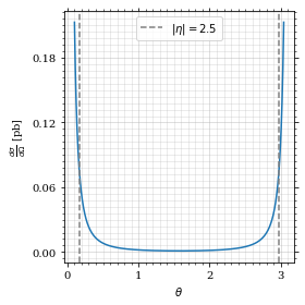

Define the integrand.

  def xs_pb_int(θ):
      return gev_to_pb(np.sin(θ)*diff_xs(θ, charge=charge, esp=esp))

Plot the integrand. # TODO: remove duplication

fig, ax = set_up_plot()
ax.plot(plot_points, xs_pb_int(plot_points))
ax.set_xlabel(r'$\theta$')
ax.set_ylabel(r'$\sin(\theta)\cdot\frac{d\sigma}{d\theta}$ [pb]')
ax.axvline(interval[0], color='gray', linestyle='--')
ax.axvline(interval[1], color='gray', linestyle='--', label=rf'$|\eta|={η}$')
ax.legend()
save_fig(fig, 'xs_integrand', 'xs', size=[4, 4])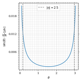

Intergrate σ with the mc method.

  xs_pb_mc, xs_pb_mc_err = integrate(xs_pb_int, interval, 10000)
  xs_pb_mc = xs_pb_mc*np.pi*2
  xs_pb_mc, xs_pb_mc_err

(0.05382327328187836, 4.2568280254619665e-05)

print(tex_value(xs_pb_mc, unit=r'\pico\barn', prefix=r'\sigma = ', prec=5))

/hiro/bachelor_thesis/src/commit/d05c1601d126d82859eb3469a9941f5eaf41e7a0/prog/python/qqgg/results/xs_mc.tex

Sampling and Analysis

Now we monte-carlo sample our distribution.

cosθ_sample = sample(lambda x: diff_xs_cosθ(x, charge, esp), interval_cosθ)
η_sample = sample(lambda x: diff_xs_eta(x, charge, esp), interval_η)
pt_sample = sample(lambda x: diff_xs_pt(x, charge, esp), interval_pt)

Nice! And now draw some histograms.

We define an auxilliary method for convenience.

  def draw_histo(points, xlabel, bins=20):
      fig, ax = set_up_plot()
      ax.hist(points, bins, histtype='step')
      ax.set_xlabel(xlabel)
      ax.set_xlim([points.min(), points.max()])
      return fig, ax

The histogram for cosθ.

fig, _ = draw_histo(cosθ_sample, r'$\cos\theta$')
save_fig(fig, 'histo_cos_theta', 'xs', size=(4,2))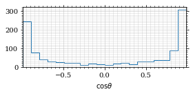

And the histogram for η.

draw_histo(η_sample, r'$\eta$')
save_fig(fig, 'histo_eta', 'xs', size=(4,2))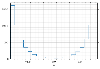

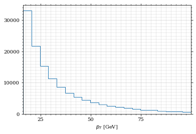
And the same for pt.

draw_histo(pt_sample, r'$p_{T}$ [GeV]')
save_fig(fig, 'histo_pt', 'xs', size=(4,2))