bachelor_thesis/prog/python/qqgg/analytical_xs.org

• Init
  • Required Modules
  • Utilities
• Implementation
• Calculations
  • Analytical Integration
  • Numerical Integration
    • Integral over θ
    • Integration over η
    • Using VEGAS
    • Testing the Statistics
  • Sampling and Analysis
    • Sampling the cosθ cross section
    • Observables
    • Sampling the η cross section

Init

Required Modules

  import numpy as np
  import matplotlib.pyplot as plt
  import monte_carlo

Utilities

%run ../utility.py
%load_ext autoreload
%aimport monte_carlo
%autoreload 1

Implementation

  """
  Implementation of the analytical cross section for q q_bar ->
  gamma gamma

  Author: Valentin Boettcher <hiro@protagon.space>
  """

  import numpy as np

  # NOTE: a more elegant solution would be a decorator
  def energy_factor(charge, esp):
      """
      Calculates the factor common to all other values in this module

      Arguments:
      esp -- center of momentum energy in GeV
      charge -- charge of the particle in units of the elementary charge
      """

      return charge**4/(137.036*esp)**2/6


  def diff_xs(θ, charge, esp):
      """
      Calculates the differential cross section as a function of the
      azimuth angle θ in units of 1/GeV².

      Here dΩ=sinθdθdφ

      Arguments:
      θ -- azimuth angle
      esp -- center of momentum energy in GeV
      charge -- charge of the particle in units of the elementary charge
      """

      f = energy_factor(charge, esp)
      return f*((np.cos(θ)**2+1)/np.sin(θ)**2)

  def diff_xs_cosθ(cosθ, charge, esp):
      """
      Calculates the differential cross section as a function of the
      cosine of the azimuth angle θ in units of 1/GeV².

      Here dΩ=d(cosθ)dφ

      Arguments:
      cosθ -- cosine of the azimuth angle
      esp -- center of momentum energy in GeV
      charge -- charge of the particle in units of the elementary charge
      """

      f = energy_factor(charge, esp)
      return f*((cosθ**2+1)/(1-cosθ**2))


  def diff_xs_eta(η, charge, esp):
      """
      Calculates the differential cross section as a function of the
      pseudo rapidity of the photons in units of 1/GeV^2.

      This is actually the crossection dσ/(dφdη).

      Arguments:
      η -- pseudo rapidity
      esp -- center of momentum energy in GeV
      charge -- charge of the particle in units of the elementary charge
      """

      f = energy_factor(charge, esp)
      return f*(np.tanh(η)**2 + 1)


  def diff_xs_p_t(p_t, charge, esp):
      """
      Calculates the differential cross section as a function of the
      transverse momentum (p_t) of the photons in units of 1/GeV^2.

      This is actually the crossection dσ/(dφdp_t).

      Arguments:
      p_t -- transverse momentum in GeV
      esp -- center of momentum energy in GeV
      charge -- charge of the particle in units of the elementary charge
      """

      f = energy_factor(charge, esp)
      sqrt_fact = np.sqrt(1-(2*p_t/esp)**2)
      return f/p_t*(1/sqrt_fact + sqrt_fact)


  def total_xs_eta(η, charge, esp):
      """
      Calculates the total cross section as a function of the pseudo
      rapidity of the photons in units of 1/GeV^2.  If the rapditiy is
      specified as a tuple, it is interpreted as an interval.  Otherwise
      the interval [-η, η] will be used.

      Arguments:
      η -- pseudo rapidity (tuple or number)
      esp -- center of momentum energy in GeV
      charge -- charge of the particle in units of the elementar charge
      """

      f = energy_factor(charge, esp)
      if not isinstance(η, tuple):
          η = (-η, η)

      if len(η) != 2:
          raise ValueError('Invalid η cut.')

      def F(x):
          return np.tanh(x) - 2*x

      return 2*np.pi*f*(F(η[0]) - F(η[1]))

Calculations

First, set up the input parameters.

η = 2.5
charge = 1/3
esp = 200  # GeV

Set up the integration and plot intervals.

interval_η = [-η, η]
interval = η_to_θ([-η, η])
interval_cosθ = np.cos(interval)
interval_pt = np.sort(η_to_pt([0, η], esp/2))
plot_interval = [0.1, np.pi-.1]

Analytical Integration

And now calculate the cross section in picobarn.

  xs_gev = total_xs_eta(η, charge, esp)
  xs_pb = gev_to_pb(xs_gev)
  tex_value(xs_pb, unit=r'\pico\barn', prefix=r'\sigma = ',
            prec=6, save=('results', 'xs.tex'))

\(\sigma = \SI{0.053793}{\pico\barn}\)

Lets plot the total xs as a function of η.

  fig, ax = set_up_plot()
  η_s = np.linspace(0, 3, 1000)
  ax.plot(η_s, gev_to_pb(total_xs_eta(η_s, charge, esp)))
  ax.set_xlabel(r'$\eta$')
  ax.set_ylabel(r'$\sigma$ [pb]')
  ax.set_xlim([0, max(η_s)])
  ax.set_ylim(0)
  save_fig(fig, 'total_xs', 'xs', size=[2.5, 2])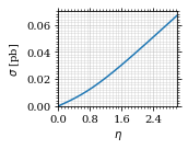

Compared to sherpa, it's pretty close.

  sherpa = 0.05380
  xs_pb - sherpa

-6.7112594623469635e-06

I had to set the runcard option EW_SCHEME: alpha0 to use the pure QED coupling constant.

Numerical Integration

Plot our nice distribution:

plot_points = np.linspace(*plot_interval, 1000)

fig, ax = set_up_plot()
ax.plot(plot_points, gev_to_pb(diff_xs(plot_points, charge=charge, esp=esp)))
ax.set_xlabel(r'$\theta$')
ax.set_ylabel(r'$d\sigma/d\Omega$ [pb]')
ax.axvline(interval[0], color='gray', linestyle='--')
ax.axvline(interval[1], color='gray', linestyle='--', label=rf'$|\eta|={η}$')
ax.legend()
save_fig(fig, 'diff_xs', 'xs', size=[2.5, 2])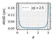

Define the integrand.

  def xs_pb_int(θ):
      return 2*np.pi*gev_to_pb(np.sin(θ)*diff_xs(θ, charge=charge, esp=esp))

  def xs_pb_int_η(η):
      return 2*np.pi*gev_to_pb(diff_xs_eta(η, charge, esp))

Plot the integrand. # TODO: remove duplication

fig, ax = set_up_plot()
ax.plot(plot_points, xs_pb_int(plot_points))
ax.set_xlabel(r'$\theta$')
ax.set_ylabel(r'$\sin(\theta)\cdot\frac{d\sigma}{d\Omega}$ [pb]')
ax.axvline(interval[0], color='gray', linestyle='--')
ax.axvline(interval[1], color='gray', linestyle='--', label=rf'$|\eta|={η}$')
ax.legend()
save_fig(fig, 'xs_integrand', 'xs', size=[4, 4])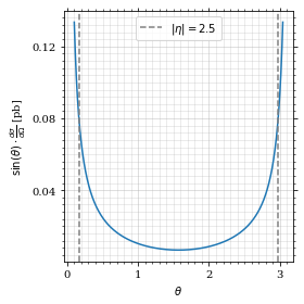

Integral over θ

Intergrate σ with the mc method.

  xs_pb_mc, xs_pb_mc_err = monte_carlo.integrate(xs_pb_int, interval, 1000)
  xs_pb_mc = xs_pb_mc
  xs_pb_mc, xs_pb_mc_err

0.05323177940348952

0.000836179760412404

We gonna export that as tex.

tex_value(xs_pb_mc, unit=r'\pico\barn', prefix=r'\sigma = ', err=xs_pb_mc_err, save=('results', 'xs_mc.tex'))

\(\sigma = \SI{0.0543\pm 0.0008}{\pico\barn}\)

Integration over η

Plot the intgrand of the pseudo rap.

fig, ax = set_up_plot()
points = np.linspace(*interval_η, 1000)
ax.plot(points, xs_pb_int_η(points))
ax.set_xlabel(r'$\eta$')
ax.set_ylabel(r'$\frac{d\sigma}{d\theta}$ [pb]')
save_fig(fig, 'xs_integrand_η', 'xs', size=[4, 4])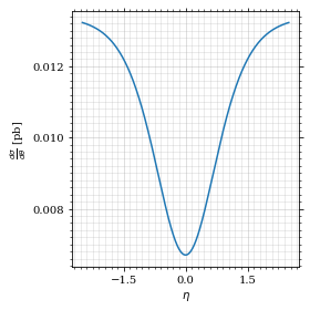

As we see, the result is much better if we use pseudo rapidity, because the differential cross section does not difverge anymore.

  xs_pb_η = monte_carlo.integrate(xs_pb_int_η,
                                  interval_η, 1000)
  xs_pb_η

0.05369352543075011

0.0001566582384086374

And yet again export that as tex.

tex_value(*xs_pb_η, unit=r'\pico\barn', prefix=r'\sigma = ', save=('results', 'xs_mc_eta.tex'))

\(\sigma = \SI{0.05398\pm 0.00016}{\pico\barn}\)

Using VEGAS

Now we use VEGAS on the θ parametrisation and see what happens.

  xs_pb_vegas, xs_pb_vegas_σ, xs_θ_intervals = \
      monte_carlo.integrate_vegas(xs_pb_int, interval,
                                  num_increments=20, alpha=4,
                                  point_density=1000, acumulate=True)
  xs_pb_vegas, xs_pb_vegas_σ

shtsh

0.053806254940947366

5.91849792512895e-05

This is pretty good, although the variance reduction may be achieved partially by accumulating the results from all runns. The uncertainty is being overestimated!

And export that as tex.

  tex_value(xs_pb_vegas, xs_pb_vegas_σ, unit=r'\pico\barn',
            prefix=r'\sigma = ', save=('results', 'xs_mc_θ_vegas.tex'))

\(\sigma = \SI{0.05383\pm 0.00007}{\pico\barn}\)

Surprisingly, without acumulation, the result ain't much different. This depends, of course, on the iteration count.

  monte_carlo.integrate_vegas(xs_pb_int, interval, num_increments=20,
                              alpha=4, point_density=1000,
                              acumulate=False)[0:2]

0.05386167571815434

7.519896920354165e-05

Testing the Statistics

Let's battle test the statistics.

  num_runs = 1000
  num_within = 0

  for _ in range(num_runs):
      val, err = monte_carlo.integrate(xs_pb_int_η, interval_η, 1000)
      if abs(xs_pb - val) <= err:
          num_within += 1

  num_within/num_runs

0.671

So we see: the standard deviation is sound.

Doing the same thing with VEGAS shows, that we overestimate σ here.

    num_runs = 1000
    num_within = 0

    for _ in range(num_runs):
        val, err, _ = \
            monte_carlo.integrate_vegas(xs_pb_int, interval,
                                        num_increments=20, alpha=4,
                                        point_density=1000, acumulate=False)
        if abs(xs_pb - val) <= err:
            num_within += 1

    num_within/num_runs

0.727

Sampling and Analysis

Define the sample number.

  sample_num = 1000

Let's define shortcuts for our distributions. The 2π are just there for formal correctnes. Factors do not influecence the outcome.

  def dist_θ(x):
      return gev_to_pb(diff_xs_cosθ(x, charge, esp))*2*np.pi

  def dist_η(x):
      return gev_to_pb(diff_xs_eta(x, charge, esp))*2*np.pi

Sampling the cosθ cross section

Now we monte-carlo sample our distribution. We observe that the efficiency his very bad!

  cosθ_sample, cosθ_efficiency = \
      monte_carlo.sample_unweighted_array(sample_num, dist_θ,
                                          interval_cosθ, report_efficiency=True)
  cosθ_efficiency

0.026983702912102593

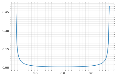
Our distribution has a lot of variance, as can be seen by plotting it.

    pts = np.linspace(*interval_cosθ, 100)
    fig, ax = set_up_plot()
    ax.plot(pts, dist_θ(pts), label=r'$\frac{d\sigma}{d\Omega}$')

<matplotlib.lines.Line2D

at

0x7f71fa2accd0>

We define a friendly and easy to integrate upper limit function.

  upper_limit = dist_θ(interval_cosθ[0]) \
      /interval_cosθ[0]**2
  upper_base = dist_θ(0)

  def upper(x):
      return  upper_base + upper_limit*x**2

  def upper_int(x):
      return  upper_base*x + upper_limit*x**3/3

  ax.plot(pts, upper(pts), label='Upper bound')
  ax.legend()
  ax.set_xlabel(r'$\cos\theta$')
  ax.set_ylabel(r'$\frac{d\sigma}{d\Omega}$')
  save_fig(fig, 'upper_bound', 'xs_sampling', size=(4, 4))
  fig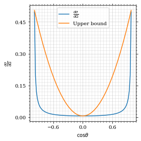

To increase our efficiency, we have to specify an upper bound. That is at least a little bit better. The numeric inversion is horribly inefficent.

  cosθ_sample, cosθ_efficiency = \
      monte_carlo.sample_unweighted_array(sample_num, dist_θ,
                                          interval_cosθ, report_efficiency=True,
                                          upper_bound=[upper, upper_int])
  cosθ_efficiency

0.08121827411167512

Nice! And now draw some histograms.

We define an auxilliary method for convenience.

  import matplotlib.pyplot as plt

  def draw_histo(points, xlabel, bins=20):
      heights, edges = np.histogram(points, bins)
      centers = (edges[1:] + edges[:-1])/2
      deviations = np.sqrt(heights)

      fig, ax = set_up_plot()
      ax.errorbar(centers, heights, deviations, linestyle='none', color='orange')
      ax.step(edges,  [heights[0], *heights], color='#1f77b4')

      ax.set_xlabel(xlabel)
      ax.set_xlim([points.min(), points.max()])
      return fig, ax

The histogram for cosθ.

fig, _ = draw_histo(cosθ_sample, r'$\cos\theta$')
save_fig(fig, 'histo_cos_theta', 'xs', size=(4,3))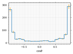

Observables

Now we define some utilities to draw real 4-momentum samples.

  def sample_momenta(sample_num, interval, charge, esp, seed=None):
      """Samples `sample_num` unweighted photon 4-momenta from the
      cross-section.

      :param sample_num: number of samples to take
      :param interval: cosθ interval to sample from
      :param charge: the charge of the quark
      :param esp: center of mass energy
      :param seed: the seed for the rng, optional, default is system
          time

      :returns: an array of 4 photon momenta

      :rtype: np.ndarray
      """
      cosθ_sample = \
          monte_carlo.sample_unweighted_array(sample_num,
                                              lambda x:
                                                diff_xs_cosθ(x, charge, esp),
                                             interval_cosθ)
      φ_sample = np.random.uniform(0, 1, sample_num)

      def make_momentum(esp, cosθ, φ):
          sinθ = np.sqrt(1-cosθ**2)
          return np.array([1, sinθ*np.cos(φ), sinθ*np.sin(φ), cosθ])*esp/2

      momenta = np.array([make_momentum(esp, cosθ, φ) \
                           for cosθ, φ in np.array([cosθ_sample, φ_sample]).T])
      return momenta

To generate histograms of other obeservables, we have to define them as functions on 4-impuleses. Using those to transform samples is analogous to transforming the distribution itself.

  """This module defines some observables on arrays of 4-pulses."""
  import numpy as np

  def p_t(p):
      """Transverse momentum

      :param p: array of 4-momenta
      """

      return np.linalg.norm(p[:,1:3], axis=1)

  def η(p):
      """Pseudo rapidity.

      :param p: array of 4-momenta
      """

      return np.arccosh(np.linalg.norm(p[:,1:], axis=1)/p_t(p))*np.sign(p[:, 3])

Lets try it out.

  momentum_sample = sample_momenta(2000, interval_cosθ, charge, esp)
  momentum_sample

array([[100.        ,  14.99955553,   6.52933179, -98.65283149],
       [100.        ,  48.11160501,  71.52596373, -50.68836134],
       [100.        ,  27.36251906,   1.55938536, -96.17099806],
       ...,
       [100.        ,  98.44690501,  13.80044529,  10.85147935],
       [100.        ,  17.20635886,   4.27420589,  98.41581366],
       [100.        ,  66.84034758,  32.63142055,  66.83979599]])

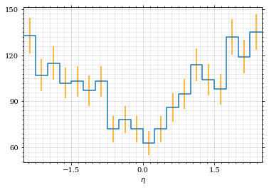
Now let's make a histogram of the η distribution.

  η_sample = η(momentum_sample)
  draw_histo(η_sample, r'$\eta$')

<Figure

size

432x288

with

1

Axes>

<matplotlib.axes._subplots.AxesSubplot

at

0x7f71fa804310>

And the same for the p_t (transverse momentum) distribution.

  p_t_sample = p_t(momentum_sample)
  draw_histo(p_t_sample, r'$p_T$ [GeV]')

<Figure

size

432x288

with

1

Axes>

<matplotlib.axes._subplots.AxesSubplot

at

0x7f71fa8a4250>

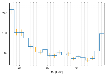
That looks somewhat fishy, but it isn't.

  fig, ax = set_up_plot()
  points = np.linspace(interval_pt[0], interval_pt[1] - .01, 1000)
  ax.plot(points, gev_to_pb(diff_xs_p_t(points, charge, esp)))
  ax.set_xlabel(r'$p_T$')
  ax.set_xlim(interval_pt[0], interval_pt[1] + 1)
  ax.set_ylim([0, gev_to_pb(diff_xs_p_t(interval_pt[1] -.01, charge, esp))])
  ax.set_ylabel(r'$\frac{d\sigma}{dp_t}$ [pb]')
  save_fig(fig, 'diff_xs_p_t', 'xs_sampling', size=[4, 3])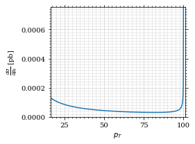

this is strongly peaked at p_t=100GeV. (The jacobian goes like 1/x there!)

Sampling the η cross section

An again we see that the efficiency is way, way! better…

  η_sample, η_efficiency = \
      monte_carlo.sample_unweighted_array(sample_num, dist_η,
                                          interval_η, report_efficiency=True)
  η_efficiency

0.3973333333333333

Let's draw a histogram to compare with the previous results.

  draw_histo(η_sample, r'$\eta$')

<Figure

size

432x288

with

1

Axes>

<matplotlib.axes._subplots.AxesSubplot

at

0x7f71fa59e820>

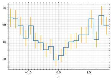
Looks good to me :).