11 KiB
Init
Required Modules
  import numpy as np
  import matplotlib.pyplot as plt
  import monte_carlo
Utilities
%run ../utility.py
%load_ext autoreload
%aimport monte_carlo
%autoreload 1
Implementation
  """
  Implementation of the analytical cross section for q q_bar ->
  gamma gamma

  Author: Valentin Boettcher <hiro@protagon.space>
  """

  import numpy as np
  from scipy.constants import alpha

  # NOTE: a more elegant solution would be a decorator
  def energy_factor(charge, esp):
      """
      Calculates the factor common to all other values in this module

      Arguments:
      esp -- center of momentum energy in GeV
      charge -- charge of the particle in units of the elementary charge
      """

      return charge**4*(alpha/esp)**2/6


  def diff_xs(θ, charge, esp):
      """
      Calculates the differential cross section as a function of the
      azimuth angle θ in units of 1/GeV².

      Arguments:
      θ -- azimuth angle
      esp -- center of momentum energy in GeV
      charge -- charge of the particle in units of the elementary charge
      """

      f = energy_factor(charge, esp)
      return f*((np.cos(θ)**2+1)/np.sin(θ)**2)

  def diff_xs_cosθ(cosθ, charge, esp):
      """
      Calculates the differential cross section as a function of the
      cosine of the azimuth angle θ in units of 1/GeV².

      Arguments:
      cosθ -- cosine of the azimuth angle
      esp -- center of momentum energy in GeV
      charge -- charge of the particle in units of the elementary charge
      """

      f = energy_factor(charge, esp)
      return f*((cosθ**2+1)/(1-cosθ**2))

  def diff_xs_eta(η, charge, esp):
      """
      Calculates the differential cross section as a function of the
      pseudo rapidity of the photons in units of 1/GeV^2.

      Arguments:
      η -- pseudo rapidity
      esp -- center of momentum energy in GeV
      charge -- charge of the particle in units of the elementary charge
      """

      f = energy_factor(charge, esp)
      return f*(2*np.cosh(η)**2 - 1)

  def diff_xs_pt(pt, charge, esp):
      """
      Calculates the differential cross section as a function of the
      transversal impulse of the photons in units of 1/GeV^2.

      Arguments:
      η -- transversal impulse
      esp -- center of momentum energy in GeV
      charge -- charge of the particle in units of the elementary charge
      """

      f = energy_factor(charge, esp)
      return f*((esp/pt)**2/2 - 1)

  def total_xs_eta(η, charge, esp):
      """
      Calculates the total cross section as a function of the pseudo
      rapidity of the photons in units of 1/GeV^2.  If the rapditiy is
      specified as a tuple, it is interpreted as an interval.  Otherwise
      the interval [-η, η] will be used.

      Arguments:
      η -- pseudo rapidity (tuple or number)
      esp -- center of momentum energy in GeV
      charge -- charge of the particle in units of the elementar charge
      """

      f = energy_factor(charge, esp)
      if not isinstance(η, tuple):
          η = (-η, η)

      if len(η) != 2:
          raise ValueError('Invalid η cut.')

      def F(x):
          return np.tanh(x) - 2*x

      return 2*np.pi*f*(F(η[0]) - F(η[1]))
Calculations
XS qq -> gamma gamma
First, set up the input parameters.
η = 2.5
charge = 1/3
esp = 200  # GeV
Set up the integration and plot intervals.
interval_η = [-η, η]
interval = η_to_θ([-η, η])
interval_cosθ = np.cos(interval)
interval_pt = η_to_pt([0, η], esp/2)
plot_interval = [0.1, np.pi-.1]
Analytical Integratin
And now calculate the cross section in picobarn.
  xs_gev = total_xs_eta(η, charge, esp)
  xs_pb = gev_to_pb(xs_gev)
  print(tex_value(xs_pb, unit=r'\pico\barn', prefix=r'\sigma = ', prec=5))
\(\sigma = \SI{0.05379}{\pico\barn}\)
Compared to sherpa, it's pretty close.
  sherpa = 0.0538009
  xs_pb/sherpa
0.9998585425137037
I had to set the runcard option EW_SCHEME: alpha0 to use the pure
QED coupling constant.
Numerical Integration
Plot our nice distribution:
plot_points = np.linspace(*plot_interval, 1000)

fig, ax = set_up_plot()
ax.plot(plot_points, gev_to_pb(diff_xs(plot_points, charge=charge, esp=esp)))
ax.set_xlabel(r'$\theta$')
ax.set_ylabel(r'$\frac{d\sigma}{d\Omega}$ [pb]')
ax.axvline(interval[0], color='gray', linestyle='--')
ax.axvline(interval[1], color='gray', linestyle='--', label=rf'$|\eta|={η}$')
ax.legend()
save_fig(fig, 'diff_xs', 'xs', size=[4, 4])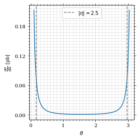
Define the integrand.
  def xs_pb_int(θ):
      return gev_to_pb(np.sin(θ)*diff_xs(θ, charge=charge, esp=esp))
Plot the integrand. # TODO: remove duplication
fig, ax = set_up_plot()
ax.plot(plot_points, xs_pb_int(plot_points))
ax.set_xlabel(r'$\theta$')
ax.set_ylabel(r'$\sin(\theta)\cdot\frac{d\sigma}{d\theta}$ [pb]')
ax.axvline(interval[0], color='gray', linestyle='--')
ax.axvline(interval[1], color='gray', linestyle='--', label=rf'$|\eta|={η}$')
ax.legend()
save_fig(fig, 'xs_integrand', 'xs', size=[4, 4])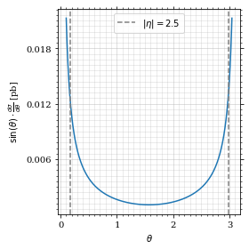
Intergrate σ with the mc method.
  xs_pb_mc, xs_pb_mc_err = monte_carlo.integrate(xs_pb_int, interval, 10000)
  xs_pb_mc = xs_pb_mc*np.pi*2
xs_pb_mc, xs_pb_mc_err| 0.05365000636562272 | 4.2342293364016736e-05 |
We gonna export that as tex.
print(tex_value(xs_pb_mc, unit=r'\pico\barn', prefix=r'\sigma = ', prec=5))\(\sigma = \SI{0.05365}{\pico\barn}\)
Sampling and Analysis
Define the sample number.
sample_num = 1000Now we monte-carlo sample our distribution.
cosθ_sample = monte_carlo.sample_unweighted_array(sample_num, lambda x:
                                            diff_xs_cosθ(x, charge, esp),
                                            interval_cosθ)
Nice! And now draw some histograms.
We define an auxilliary method for convenience.
  def draw_histo(points, xlabel, bins=20):
      fig, ax = set_up_plot()
      ax.hist(points, bins, histtype='step')
      ax.set_xlabel(xlabel)
      ax.set_xlim([points.min(), points.max()])
      return fig, ax
The histogram for cosθ.
fig, _ = draw_histo(cosθ_sample, r'$\cos\theta$')
save_fig(fig, 'histo_cos_theta', 'xs', size=(4,3))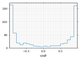
Now we define some utilities to draw real 4-impulse samples.
  def sample_impulses(sample_num, interval, charge, esp, seed=None):
      """Samples `sample_num` unweighted photon 4-impulses from the cross-section.

      :param sample_num: number of samples to take
      :param interval: cosθ interval to sample from
      :param charge: the charge of the quark
      :param esp: center of mass energy
      :param seed: the seed for the rng, optional, default is system
          time

      :returns: an array of 4 photon impulses
      :rtype: np.ndarray
      """
      cosθ_sample = \
          monte_carlo.sample_unweighted_array(sample_num,
                                              lambda x:
                                                diff_xs_cosθ(x, charge, esp),
                                             interval_cosθ)
      φ_sample = np.random.uniform(0, 1, sample_num)

      def make_impulse(esp, cosθ, φ):
          sinθ = np.sqrt(1-cosθ**2)
          return np.array([1, sinθ*np.cos(φ), sinθ*np.sin(φ), cosθ])*esp/2

      impulses = np.array([make_impulse(esp, cosθ, φ) \
                           for cosθ, φ in np.array([cosθ_sample, φ_sample]).T])
      return impulses
To generate histograms of other obeservables, we have to define them as functions on 4-impuleses. Using those to transform samples is analogous to transforming the distribution itself.
  """This module defines some observables on arrays of 4-pulses."""
  import numpy as np

  def p_t(p):
      """Transverse impulse

      :param p: array of 4-impulses
      """

      return np.linalg.norm(p[:,1:3], axis=1)

  def η(p):
      """Pseudo rapidity.

      :param p: array of 4-impulses
      """

      return np.arccosh(np.linalg.norm(p[:,1:], axis=1)/p_t(p))*np.sign(p[:, 3])
Lets try it out.
  impulse_sample = sample_impulses(2000, interval_cosθ, charge, esp)
  impulse_sample
array([[100. , 60.93780026, 38.29391655, 69.42737539],
[100. , 16.62473755, 5.08308744, -98.47730867],
[100. , 62.52584971, 41.05712399, 66.3688985 ],
...,
[100. , 36.93115123, 10.77808502, -92.30342871],
[100. , 34.39831699, 43.0134429 , 83.46615792],
[100. , 69.87424822, 3.87926805, 71.43207063]])
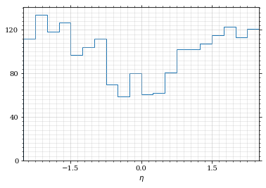
Now let's make a histogram of the η distribution.
  η_sample = η(impulse_sample)
draw_histo(η_sample, r'$\eta$')| <Figure | size | 432x288 | with | 1 | Axes> | <matplotlib.axes._subplots.AxesSubplot | at | 0x7fb464af2040> |
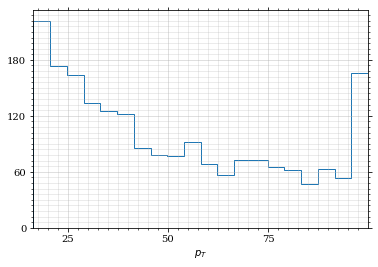
And the same for the p_t (transverse impulse) distribution.
  p_t_sample = p_t(impulse_sample)
draw_histo(p_t_sample, r'$p_T$')| <Figure | size | 432x288 | with | 1 | Axes> | <matplotlib.axes._subplots.AxesSubplot | at | 0x7fb463469d60> |