bachelor_thesis/prog/python/qqgg/analytical_xs.org

Investigaton of Monte-Carlo Methods

• Init
  • Required Modules
  • Utilities
• Implementation
• Calculations
  • Analytical Integration
  • Numerical Integration
    • Integral over θ
    • Integration over η
    • Using VEGAS
    • Testing the Statistics
  • Sampling and Analysis
    • Sampling the cosθ cross section
    • Observables
    • Sampling the η cross section
    • Sampling with VEGAS

Init

Required Modules

  import numpy as np
  import matplotlib.pyplot as plt
  import monte_carlo

Utilities

%run ../utility.py
%load_ext autoreload
%aimport monte_carlo
%autoreload 1

The autoreload extension is already loaded. To reload it, use:
  %reload_ext autoreload

Implementation

  """
  Implementation of the analytical cross section for q q_bar ->
  gamma gamma

  Author: Valentin Boettcher <hiro@protagon.space>
  """

  import numpy as np

  # NOTE: a more elegant solution would be a decorator
  def energy_factor(charge, esp):
      """
      Calculates the factor common to all other values in this module

      Arguments:
      esp -- center of momentum energy in GeV
      charge -- charge of the particle in units of the elementary charge
      """

      return charge**4/(137.036*esp)**2/6


  def diff_xs(θ, charge, esp):
      """
      Calculates the differential cross section as a function of the
      azimuth angle θ in units of 1/GeV².

      Here dΩ=sinθdθdφ

      Arguments:
      θ -- azimuth angle
      esp -- center of momentum energy in GeV
      charge -- charge of the particle in units of the elementary charge
      """

      f = energy_factor(charge, esp)
      return f*((np.cos(θ)**2+1)/np.sin(θ)**2)

  def diff_xs_cosθ(cosθ, charge, esp):
      """
      Calculates the differential cross section as a function of the
      cosine of the azimuth angle θ in units of 1/GeV².

      Here dΩ=d(cosθ)dφ

      Arguments:
      cosθ -- cosine of the azimuth angle
      esp -- center of momentum energy in GeV
      charge -- charge of the particle in units of the elementary charge
      """

      f = energy_factor(charge, esp)
      return f*((cosθ**2+1)/(1-cosθ**2))


  def diff_xs_eta(η, charge, esp):
      """
      Calculates the differential cross section as a function of the
      pseudo rapidity of the photons in units of 1/GeV^2.

      This is actually the crossection dσ/(dφdη).

      Arguments:
      η -- pseudo rapidity
      esp -- center of momentum energy in GeV
      charge -- charge of the particle in units of the elementary charge
      """

      f = energy_factor(charge, esp)
      return f*(np.tanh(η)**2 + 1)


  def diff_xs_p_t(p_t, charge, esp):
      """
      Calculates the differential cross section as a function of the
      transverse momentum (p_t) of the photons in units of 1/GeV^2.

      This is actually the crossection dσ/(dφdp_t).

      Arguments:
      p_t -- transverse momentum in GeV
      esp -- center of momentum energy in GeV
      charge -- charge of the particle in units of the elementary charge
      """

      f = energy_factor(charge, esp)
      sqrt_fact = np.sqrt(1-(2*p_t/esp)**2)
      return f/p_t*(1/sqrt_fact + sqrt_fact)


  def total_xs_eta(η, charge, esp):
      """
      Calculates the total cross section as a function of the pseudo
      rapidity of the photons in units of 1/GeV^2.  If the rapditiy is
      specified as a tuple, it is interpreted as an interval.  Otherwise
      the interval [-η, η] will be used.

      Arguments:
      η -- pseudo rapidity (tuple or number)
      esp -- center of momentum energy in GeV
      charge -- charge of the particle in units of the elementar charge
      """

      f = energy_factor(charge, esp)
      if not isinstance(η, tuple):
          η = (-η, η)

      if len(η) != 2:
          raise ValueError('Invalid η cut.')

      def F(x):
          return np.tanh(x) - 2*x

      return 2*np.pi*f*(F(η[0]) - F(η[1]))

Calculations

First, set up the input parameters.

η = 2.5
charge = 1/3
esp = 200  # GeV

Set up the integration and plot intervals.

interval_η = [-η, η]
interval = η_to_θ([-η, η])
interval_cosθ = np.cos(interval)
interval_pt = np.sort(η_to_pt([0, η], esp/2))
plot_interval = [0.1, np.pi-.1]

Note that we could utilize the symetry of the integrand throughout, but that doen't reduce variance and would complicate things now.

Analytical Integration

And now calculate the cross section in picobarn.

  xs_gev = total_xs_eta(η, charge, esp)
  xs_pb = gev_to_pb(xs_gev)
  tex_value(xs_pb, unit=r'\pico\barn', prefix=r'\sigma = ',
            prec=6, save=('results', 'xs.tex'))

\(\sigma = \SI{0.053793}{\pico\barn}\)

Lets plot the total xs as a function of η.

  fig, ax = set_up_plot()
  η_s = np.linspace(0, 3, 1000)
  ax.plot(η_s, gev_to_pb(total_xs_eta(η_s, charge, esp)))
  ax.set_xlabel(r'$\eta$')
  ax.set_ylabel(r'$\sigma$ [pb]')
  ax.set_xlim([0, max(η_s)])
  ax.set_ylim(0)
  save_fig(fig, 'total_xs', 'xs', size=[2.5, 2.5])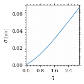

Compared to sherpa, it's pretty close.

  sherpa = 0.05380
  xs_pb - sherpa

-6.7112594623469635e-06

I had to set the runcard option EW_SCHEME: alpha0 to use the pure QED coupling constant.

Numerical Integration

Plot our nice distribution:

  plot_points = np.linspace(*plot_interval, 1000)

  fig, ax = set_up_plot()
  ax.plot(plot_points, gev_to_pb(diff_xs(plot_points, charge=charge, esp=esp)))
  ax.set_xlabel(r'$\theta$')
  ax.set_ylabel(r'$d\sigma/d\Omega$ [pb]')
  ax.set_xlim([plot_points.min(), plot_points.max()])
  ax.axvline(interval[0], color='gray', linestyle='--')
  ax.axvline(interval[1], color='gray', linestyle='--', label=rf'$|\eta|={η}$')
  ax.legend()
  save_fig(fig, 'diff_xs', 'xs', size=[2.5, 2.5])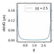

Define the integrand.

  def xs_pb_int(θ):
      return 2*np.pi*gev_to_pb(np.sin(θ)*diff_xs(θ, charge=charge, esp=esp))

  def xs_pb_int_η(η):
      return 2*np.pi*gev_to_pb(diff_xs_eta(η, charge, esp))

Plot the integrand. # TODO: remove duplication

  fig, ax = set_up_plot()
  ax.plot(plot_points, xs_pb_int(plot_points))
  ax.set_xlabel(r'$\theta$')
  ax.set_ylabel(r'$\sin(\theta)\cdot\frac{d\sigma}{d\Omega}$ [pb]')
  ax.set_xlim([plot_points.min(), plot_points.max()])
  ax.axvline(interval[0], color='gray', linestyle='--')
  ax.axvline(interval[1], color='gray', linestyle='--', label=rf'$|\eta|={η}$')
  ax.legend()
  save_fig(fig, 'xs_integrand', 'xs', size=[4, 4])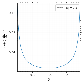

Integral over θ

Intergrate σ with the mc method.

  xs_pb_mc, xs_pb_mc_err = monte_carlo.integrate(xs_pb_int, interval, 1000)
  xs_pb_mc = xs_pb_mc
  xs_pb_mc, xs_pb_mc_err

0.05441643331124812

0.000850414167068247

We gonna export that as tex.

tex_value(xs_pb_mc, unit=r'\pico\barn', prefix=r'\sigma = ', err=xs_pb_mc_err, save=('results', 'xs_mc.tex'))

\(\sigma = \SI{0.0544\pm 0.0009}{\pico\barn}\)

Integration over η

Plot the intgrand of the pseudo rap.

fig, ax = set_up_plot()
points = np.linspace(*interval_η, 1000)
ax.plot(points, xs_pb_int_η(points))
ax.set_xlabel(r'$\eta$')
ax.set_ylabel(r'$\frac{d\sigma}{d\theta}$ [pb]')
save_fig(fig, 'xs_integrand_η', 'xs', size=[4, 4])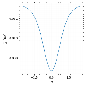

  xs_pb_η = monte_carlo.integrate(xs_pb_int_η,
                                  interval_η, 1000)
  xs_pb_η

0.05387227556308623

0.00015784230303183058

As we see, the result is a little better if we use pseudo rapidity, because the differential cross section does not difverge anymore. But becase our η interval is covering the range where all the variance is occuring, the improvement is rather marginal.

And yet again export that as tex.

  tex_value(*xs_pb_η, unit=r'\pico\barn', prefix=r'\sigma = ',
            save=('results', 'xs_mc_eta.tex'))

\(\sigma = \SI{0.05387\pm 0.00016}{\pico\barn}\)

Using VEGAS

Now we use VEGAS on the θ parametrisation and see what happens.

  xs_pb_vegas, xs_pb_vegas_σ, xs_θ_intervals = \
      monte_carlo.integrate_vegas(xs_pb_int, interval,
                                  num_increments=20, alpha=4,
                                  point_density=1000, acumulate=True)
  xs_pb_vegas, xs_pb_vegas_σ

0.05382003923613133

5.515086040159631e-05

This is pretty good, although the variance reduction may be achieved partially by accumulating the results from all runns. The uncertainty is being overestimated!

And export that as tex.

  tex_value(xs_pb_vegas, xs_pb_vegas_σ, unit=r'\pico\barn',
            prefix=r'\sigma = ', save=('results', 'xs_mc_θ_vegas.tex'))

\(\sigma = \SI{0.05382\pm 0.00006}{\pico\barn}\)

Surprisingly, without acumulation, the result ain't much different. This depends, of course, on the iteration count.

  monte_carlo.integrate_vegas(xs_pb_int, interval, num_increments=20,
                              alpha=4, point_density=1000,
                              acumulate=False)[0:2]

0.05378075568964776

7.452808684393069e-05

Testing the Statistics

Let's battle test the statistics.

  num_runs = 1000
  num_within = 0

  for _ in range(num_runs):
      val, err = monte_carlo.integrate(xs_pb_int_η, interval_η, 1000)
      if abs(xs_pb - val) <= err:
          num_within += 1

  num_within/num_runs

0.694

So we see: the standard deviation is sound.

Doing the same thing with VEGAS works as well.

  num_runs = 1000
  num_within = 0
  for _ in range(num_runs):
      val, err, _ = \
          monte_carlo.integrate_vegas(xs_pb_int, interval,
                                      num_increments=8, alpha=1,
                                      point_density=1000, acumulate=False)

      if abs(xs_pb - val) <= err:
          num_within += 1
  num_within/num_runs

0.672

Sampling and Analysis

Define the sample number.

  sample_num = 1000

Let's define shortcuts for our distributions. The 2π are just there for formal correctnes. Factors do not influecence the outcome.

  def dist_cosθ(x):
      return gev_to_pb(diff_xs_cosθ(x, charge, esp))*2*np.pi

  def dist_η(x):
      return gev_to_pb(diff_xs_eta(x, charge, esp))*2*np.pi

Sampling the cosθ cross section

Now we monte-carlo sample our distribution. We observe that the efficiency his very bad!

  cosθ_sample, cosθ_efficiency = \
      monte_carlo.sample_unweighted_array(sample_num, dist_cosθ,
                                          interval_cosθ, report_efficiency=True)
  cosθ_efficiency

0.027772146766673424

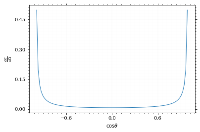
Our distribution has a lot of variance, as can be seen by plotting it.

  pts = np.linspace(*interval_cosθ, 100)
  fig, ax = set_up_plot()
  ax.plot(pts, dist_cosθ(pts))
  ax.set_xlabel(r'$\cos\theta$')
  ax.set_ylabel(r'$\frac{d\sigma}{d\Omega}$')

Text(0, 0.5, '$\\frac{d\\sigma}{d\\Omega}$')

We define a friendly and easy to integrate upper limit function.

  upper_limit = dist_cosθ(interval_cosθ[0]) \
      /interval_cosθ[0]**2
  upper_base = dist_cosθ(0)

  def upper(x):
      return  upper_base + upper_limit*x**2

  def upper_int(x):
      return  upper_base*x + upper_limit*x**3/3

  ax.plot(pts, upper(pts), label='Upper bound')
  ax.legend()
  ax.set_xlabel(r'$\cos\theta$')
  ax.set_ylabel(r'$\frac{d\sigma}{d\Omega}$')
  save_fig(fig, 'upper_bound', 'xs_sampling', size=(4, 4))
  fig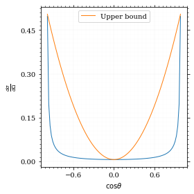

To increase our efficiency, we have to specify an upper bound. That is at least a little bit better. The numeric inversion is horribly inefficent.

  cosθ_sample, cosθ_efficiency = \
      monte_carlo.sample_unweighted_array(sample_num, dist_cosθ,
                                          interval_cosθ, report_efficiency=True,
                                          upper_bound=[upper, upper_int])
  cosθ_efficiency

0.07994628015406446

<<cosθ-bare-eff>>

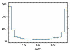
Nice! And now draw some histograms.

We define an auxilliary method for convenience.

  """
  Some shorthands for common plotting tasks related to the investigation
  of monte-carlo methods in one rimension.

  Author: Valentin Boettcher <hiro at protagon.space>
  """

  import matplotlib.pyplot as plt

  def draw_histo(points, xlabel, bins=20):
      heights, edges = np.histogram(points, bins)
      centers = (edges[1:] + edges[:-1])/2
      deviations = np.sqrt(heights)

      fig, ax = set_up_plot()
      ax.errorbar(centers, heights, deviations, linestyle='none', color='orange')
      ax.step(edges,  [heights[0], *heights], color='#1f77b4')

      ax.set_xlabel(xlabel)
      ax.set_xlim([points.min(), points.max()])
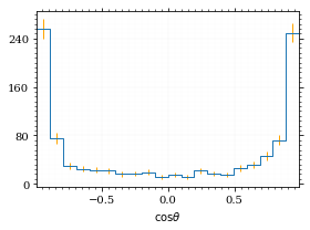
      return fig, ax

The histogram for cosθ.

fig, _ = draw_histo(cosθ_sample, r'$\cos\theta$')
save_fig(fig, 'histo_cos_theta', 'xs', size=(4,3))

  BrokenPipeErrorTraceback (most recent call last)
  <ipython-input-188-c43713624618> in <module>
        1 fig, _ = draw_histo(cosθ_sample, r'$\cos\theta$')
  ----> 2 save_fig(fig, 'histo_cos_theta', 'xs', size=(4,3))

  ~/Documents/Projects/UNI/Bachelor/prog/python/utility.py in save_fig(fig, title, folder, size)
      101
      102     fig.savefig(f'./figs/{folder}/{title}.pdf')
  --> 103     fig.savefig(f'./figs/{folder}/{title}.pgf')
      104
      105

  /usr/lib/python3.8/site-packages/matplotlib/figure.py in savefig(self, fname, transparent, **kwargs)
     2201             self.patch.set_visible(frameon)
     2202
  -> 2203         self.canvas.print_figure(fname, **kwargs)
     2204
     2205         if frameon:

  /usr/lib/python3.8/site-packages/matplotlib/backend_bases.py in print_figure(self, filename, dpi, facecolor, edgecolor, orientation, format, bbox_inches, **kwargs)
     2096
     2097             try:
  -> 2098                 result = print_method(
     2099                     filename,
     2100                     dpi=dpi,

  /usr/lib/python3.8/site-packages/matplotlib/backends/backend_pgf.py in print_pgf(self, fname_or_fh, *args, **kwargs)
      888             if not cbook.file_requires_unicode(file):
      889                 file = codecs.getwriter("utf-8")(file)
  --> 890             self._print_pgf_to_fh(file, *args, **kwargs)
      891
      892     def _print_pdf_to_fh(self, fh, *args, **kwargs):

  /usr/lib/python3.8/site-packages/matplotlib/cbook/deprecation.py in wrapper(*args, **kwargs)
      356                 f"%(removal)s.  If any parameter follows {name!r}, they "
      357                 f"should be pass as keyword, not positionally.")
  --> 358         return func(*args, **kwargs)
      359
      360     return wrapper

  /usr/lib/python3.8/site-packages/matplotlib/backends/backend_pgf.py in _print_pgf_to_fh(self, fh, dryrun, bbox_inches_restore, *args, **kwargs)
      870                                      RendererPgf(self.figure, fh),
      871                                      bbox_inches_restore=bbox_inches_restore)
  --> 872         self.figure.draw(renderer)
      873
      874         # end the pgfpicture environment

  /usr/lib/python3.8/site-packages/matplotlib/artist.py in draw_wrapper(artist, renderer, *args, **kwargs)
       36                 renderer.start_filter()
       37
  ---> 38             return draw(artist, renderer, *args, **kwargs)
       39         finally:
       40             if artist.get_agg_filter() is not None:

  /usr/lib/python3.8/site-packages/matplotlib/figure.py in draw(self, renderer)
     1733
     1734             self.patch.draw(renderer)
  -> 1735             mimage._draw_list_compositing_images(
     1736                 renderer, self, artists, self.suppressComposite)
     1737

  /usr/lib/python3.8/site-packages/matplotlib/image.py in _draw_list_compositing_images(renderer, parent, artists, suppress_composite)
      135     if not_composite or not has_images:
      136         for a in artists:
  --> 137             a.draw(renderer)
      138     else:
      139         # Composite any adjacent images together

  /usr/lib/python3.8/site-packages/matplotlib/artist.py in draw_wrapper(artist, renderer, *args, **kwargs)
       36                 renderer.start_filter()
       37
  ---> 38             return draw(artist, renderer, *args, **kwargs)
       39         finally:
       40             if artist.get_agg_filter() is not None:

  /usr/lib/python3.8/site-packages/matplotlib/axes/_base.py in draw(self, renderer, inframe)
     2628             renderer.stop_rasterizing()
     2629
  -> 2630         mimage._draw_list_compositing_images(renderer, self, artists)
     2631
     2632         renderer.close_group('axes')

  /usr/lib/python3.8/site-packages/matplotlib/image.py in _draw_list_compositing_images(renderer, parent, artists, suppress_composite)
      135     if not_composite or not has_images:
      136         for a in artists:
  --> 137             a.draw(renderer)
      138     else:
      139         # Composite any adjacent images together

  /usr/lib/python3.8/site-packages/matplotlib/artist.py in draw_wrapper(artist, renderer, *args, **kwargs)
       36                 renderer.start_filter()
       37
  ---> 38             return draw(artist, renderer, *args, **kwargs)
       39         finally:
       40             if artist.get_agg_filter() is not None:

  /usr/lib/python3.8/site-packages/matplotlib/axis.py in draw(self, renderer, *args, **kwargs)
     1226
     1227         ticks_to_draw = self._update_ticks()
  -> 1228         ticklabelBoxes, ticklabelBoxes2 = self._get_tick_bboxes(ticks_to_draw,
     1229                                                                 renderer)
     1230

  /usr/lib/python3.8/site-packages/matplotlib/axis.py in _get_tick_bboxes(self, ticks, renderer)
     1171     def _get_tick_bboxes(self, ticks, renderer):
     1172         """Return lists of bboxes for ticks' label1's and label2's."""
  -> 1173         return ([tick.label1.get_window_extent(renderer)
     1174                  for tick in ticks if tick.label1.get_visible()],
     1175                 [tick.label2.get_window_extent(renderer)

  /usr/lib/python3.8/site-packages/matplotlib/axis.py in <listcomp>(.0)
     1171     def _get_tick_bboxes(self, ticks, renderer):
     1172         """Return lists of bboxes for ticks' label1's and label2's."""
  -> 1173         return ([tick.label1.get_window_extent(renderer)
     1174                  for tick in ticks if tick.label1.get_visible()],
     1175                 [tick.label2.get_window_extent(renderer)

  /usr/lib/python3.8/site-packages/matplotlib/text.py in get_window_extent(self, renderer, dpi)
      903             raise RuntimeError('Cannot get window extent w/o renderer')
      904
  --> 905         bbox, info, descent = self._get_layout(self._renderer)
      906         x, y = self.get_unitless_position()
      907         x, y = self.get_transform().transform((x, y))

  /usr/lib/python3.8/site-packages/matplotlib/text.py in _get_layout(self, renderer)
      297             clean_line, ismath = self._preprocess_math(line)
      298             if clean_line:
  --> 299                 w, h, d = renderer.get_text_width_height_descent(
      300                     clean_line, self._fontproperties, ismath=ismath)
      301             else:

  /usr/lib/python3.8/site-packages/matplotlib/backends/backend_pgf.py in get_text_width_height_descent(self, s, prop, ismath)
      755
      756         # get text metrics in units of latex pt, convert to display units
  --> 757         w, h, d = (LatexManager._get_cached_or_new()
      758                    .get_width_height_descent(s, prop))
      759         # TODO: this should be latex_pt_to_in instead of mpl_pt_to_in

  /usr/lib/python3.8/site-packages/matplotlib/backends/backend_pgf.py in get_width_height_descent(self, text, prop)
      356
      357         # send textbox to LaTeX and wait for prompt
  --> 358         self._stdin_writeln(textbox)
      359         try:
      360             self._expect_prompt()

  /usr/lib/python3.8/site-packages/matplotlib/backends/backend_pgf.py in _stdin_writeln(self, s)
      257         self.latex_stdin_utf8.write(s)
      258         self.latex_stdin_utf8.write("\n")
  --> 259         self.latex_stdin_utf8.flush()
      260
      261     def _expect(self, s):

  BrokenPipeError: [Errno 32] Broken pipe

Observables

Now we define some utilities to draw real 4-momentum samples.

  def sample_momenta(sample_num, interval, charge, esp, seed=None):
      """Samples `sample_num` unweighted photon 4-momenta from the
      cross-section.

      :param sample_num: number of samples to take
      :param interval: cosθ interval to sample from
      :param charge: the charge of the quark
      :param esp: center of mass energy
      :param seed: the seed for the rng, optional, default is system
          time

      :returns: an array of 4 photon momenta

      :rtype: np.ndarray
      """
      cosθ_sample = \
          monte_carlo.sample_unweighted_array(sample_num,
                                              lambda x:
                                                diff_xs_cosθ(x, charge, esp),
                                             interval_cosθ)
      φ_sample = np.random.uniform(0, 1, sample_num)

      def make_momentum(esp, cosθ, φ):
          sinθ = np.sqrt(1-cosθ**2)
          return np.array([1, sinθ*np.cos(φ), sinθ*np.sin(φ), cosθ])*esp/2

      momenta = np.array([make_momentum(esp, cosθ, φ) \
                           for cosθ, φ in np.array([cosθ_sample, φ_sample]).T])
      return momenta

To generate histograms of other obeservables, we have to define them as functions on 4-impuleses. Using those to transform samples is analogous to transforming the distribution itself.

  """This module defines some observables on arrays of 4-pulses."""
  import numpy as np

  def p_t(p):
      """Transverse momentum

      :param p: array of 4-momenta
      """

      return np.linalg.norm(p[:,1:3], axis=1)

  def η(p):
      """Pseudo rapidity.

      :param p: array of 4-momenta
      """

      return np.arccosh(np.linalg.norm(p[:,1:], axis=1)/p_t(p))*np.sign(p[:, 3])

And import them.

  %aimport tangled.observables
  obs = tangled.observables

Lets try it out.

  momentum_sample = sample_momenta(2000, interval_cosθ, charge, esp)
  momentum_sample

array([[100.        ,  38.24641519,  22.76579296,  89.5484807 ],
       [100.        ,  48.14652483,  29.97226738, -82.36246314],
       [100.        ,  65.02515029,  25.82470275, -71.44798498],
       ...,
       [100.        ,  77.44294062,  27.84365663,  56.80952151],
       [100.        ,  51.47029015,  16.47983968,  84.13812522],
       [100.        ,  40.1313622 ,  23.07278301, -88.64039966]])

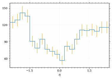
Now let's make a histogram of the η distribution.

  η_sample = obs.η(momentum_sample)
  draw_histo(η_sample, r'$\eta$')

<Figure

size

432x288

with

1

Axes>

<matplotlib.axes._subplots.AxesSubplot

at

0x7f9f4c6f0700>

And the same for the p_t (transverse momentum) distribution.

  p_t_sample = obs.p_t(momentum_sample)
  draw_histo(p_t_sample, r'$p_T$ [GeV]')

<Figure

size

432x288

with

1

Axes>

<matplotlib.axes._subplots.AxesSubplot

at

0x7f9f4c266f40>

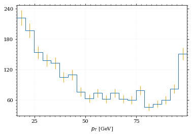
That looks somewhat fishy, but it isn't.

  fig, ax = set_up_plot()
  points = np.linspace(interval_pt[0], interval_pt[1] - .01, 1000)
  ax.plot(points, gev_to_pb(diff_xs_p_t(points, charge, esp)))
  ax.set_xlabel(r'$p_T$')
  ax.set_xlim(interval_pt[0], interval_pt[1] + 1)
  ax.set_ylim([0, gev_to_pb(diff_xs_p_t(interval_pt[1] -.01, charge, esp))])
  ax.set_ylabel(r'$\frac{d\sigma}{dp_t}$ [pb]')
  save_fig(fig, 'diff_xs_p_t', 'xs_sampling', size=[4, 3])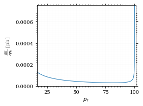

this is strongly peaked at p_t=100GeV. (The jacobian goes like 1/x there!)

Sampling the η cross section

An again we see that the efficiency is way, way! better…

  η_sample, η_efficiency = \
      monte_carlo.sample_unweighted_array(sample_num, dist_η,
                                          interval_η, report_efficiency=True)
  η_efficiency

0.4063

<<η-eff>>

Let's draw a histogram to compare with the previous results.

  draw_histo(η_sample, r'$\eta$')

<Figure

size

432x288

with

1

Axes>

<matplotlib.axes._subplots.AxesSubplot

at

0x7f9f4bdf4310>

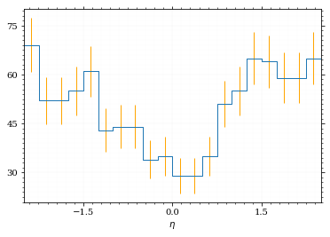
Looks good to me :).

Sampling with VEGAS

Let's define some little helpers.

  def plot_increments(ax, increment_borders, label=None, *args, **kwargs):
      """Plot the increment borders from a list.  The first and last one

      :param ax: the axis on which to draw
      :param list increment_borders: the borders of the increments
      :param str label: the label to apply to one of the vertical lines
      """

      ax.axvline(x=increment_borders[1], label=label, *args, **kwargs)

      for increment in increment_borders[2:-1]:
          ax.axvline(x=increment, *args, **kwargs)

  def plot_vegas_weighted_distribution(ax, points, dist,
                                       increment_borders, *args, **kwargs):
      """Plot the distribution with VEGAS weights applied.

      :param ax: axis
      :param points: points
      :param dist: distribution
      :param increment_borders: increment borders
      """

      num_increments = increment_borders.size
      weighted_dist = dist.copy()

      for left_border, right_border in zip(increment_borders[:-1],
                                          increment_borders[1:]):
          length = right_border - left_border
          mask = (left_border <= points) & (points <= right_border)
          weighted_dist[mask] = dist[mask]*num_increments*length

      ax.plot(points, weighted_dist, *args, **kwargs)

To get the increments, we have to let VEGAS loose on our distribution. We throw away the integral, but keep the increments.

  _, _, increments = monte_carlo.integrate_vegas(dist_cosθ,
                                                 interval_cosθ,
                                                 num_increments=10, alpha=1,
                                                 epsilon=.01)
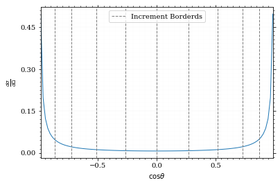
  increments

array([-0.9866143 , -0.87001384, -0.7269742 , -0.51294698, -0.26484439,
        0.00164873,  0.26764024,  0.5151555 ,  0.72867548,  0.87054888,
        0.9866143 ])

Visualizing the increment borders gives us the information we want.

  pts = np.linspace(*interval_cosθ, 100)
  fig, ax = set_up_plot()
  ax.plot(pts, dist_cosθ(pts))
  ax.set_xlabel(r'$\cos\theta$')
  ax.set_ylabel(r'$\frac{d\sigma}{d\Omega}$')
  ax.set_xlim(*interval_cosθ)
  plot_increments(ax, increments,
                  label='Increment Borderds', color='gray', linestyle='--')
  ax.legend()

<matplotlib.legend.Legend at 0x7f9f4bdd9940>

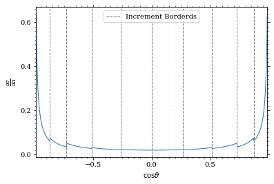
We can now plot the reweighted distribution to observe the variance reduction visually.

  pts = np.linspace(*interval_cosθ, 1000)
  fig, ax = set_up_plot()
  plot_vegas_weighted_distribution(ax, pts, dist_cosθ(pts), increments)
  ax.set_xlabel(r'$\cos\theta$')
  ax.set_ylabel(r'$\frac{d\sigma}{d\Omega}$')
  ax.set_xlim(*interval_cosθ)
  plot_increments(ax, increments,
                  label='Increment Borderds', color='gray', linestyle='--')
  ax.legend()

<matplotlib.legend.Legend at 0x7f9f4bb7ebb0>

I am batman! Now, draw a sample and look at the efficiency.

  cosθ_sample_strat, cosθ_efficiency_strat = \
      monte_carlo.sample_unweighted_array(sample_num, dist_cosθ,
                                          increment_borders=increments,
                                          report_efficiency=True)
  cosθ_efficiency_strat

0.0913

If we compare that to /hiro/bachelor_thesis/src/commit/6b5540935660e89d9e7f22476debe56214fcae65/prog/python/qqgg/cos%CE%B8-bare-eff, we can see the improvement :P. It is even better the /hiro/bachelor_thesis/src/commit/6b5540935660e89d9e7f22476debe56214fcae65/prog/python/qqgg/%CE%B7-eff. The histogram looks just the same.

fig, _ = draw_histo(cosθ_sample_strat, r'$\cos\theta$')
save_fig(fig, 'histo_cos_theta_strat', 'xs', size=(4,3))