bachelor_thesis/prog/python/qqgg/analytical_xs.org

Investigaton of Monte-Carlo Methods

• Init
  • Required Modules
  • Utilities
• Implementation
  • Center of Mass Frame
• Calculations
  • Analytical Integration
  • Numerical Integration
    • Integral over θ
    • Integration over η
    • Using VEGAS
    • Testing the Statistics
  • Sampling and Analysis
    • Sampling the cosθ cross section
    • Observables
    • Sampling the η cross section
    • Sampling with VEGAS
    • Some Histograms with Rivet
      • Init
      • Plot the Histos

Init

Required Modules

  import numpy as np
  import matplotlib.pyplot as plt
  import monte_carlo

Utilities

%run ../utility.py
%load_ext autoreload
%aimport monte_carlo
%autoreload 1

Implementation

Center of Mass Frame

  """
  Implementation of the analytical cross section for q q_bar ->
  gamma gamma

  Author: Valentin Boettcher <hiro@protagon.space>
  """

  import numpy as np

  # NOTE: a more elegant solution would be a decorator
  def energy_factor(charge, esp):
      """
      Calculates the factor common to all other values in this module

      Arguments:
      esp -- center of momentum energy in GeV
      charge -- charge of the particle in units of the elementary charge
      """

      return charge ** 4 / (137.036 * esp) ** 2 / 6


  def diff_xs(θ, charge, esp):
      """
      Calculates the differential cross section as a function of the
      azimuth angle θ in units of 1/GeV².

      Here dΩ=sinθdθdφ

      Arguments:
      θ -- azimuth angle
      esp -- center of momentum energy in GeV
      charge -- charge of the particle in units of the elementary charge
      """

      f = energy_factor(charge, esp)
      return f * ((np.cos(θ) ** 2 + 1) / np.sin(θ) ** 2)


  def diff_xs_cosθ(cosθ, charge, esp):
      """
      Calculates the differential cross section as a function of the
      cosine of the azimuth angle θ in units of 1/GeV².

      Here dΩ=d(cosθ)dφ

      Arguments:
      cosθ -- cosine of the azimuth angle
      esp -- center of momentum energy in GeV
      charge -- charge of the particle in units of the elementary charge
      """

      f = energy_factor(charge, esp)
      return f * ((cosθ ** 2 + 1) / (1 - cosθ ** 2))


  def diff_xs_eta(η, charge, esp):
      """
      Calculates the differential cross section as a function of the
      pseudo rapidity of the photons in units of 1/GeV^2.

      This is actually the crossection dσ/(dφdη).

      Arguments:
      η -- pseudo rapidity
      esp -- center of momentum energy in GeV
      charge -- charge of the particle in units of the elementary charge
      """

      f = energy_factor(charge, esp)
      return f * (np.tanh(η) ** 2 + 1)


  def diff_xs_p_t(p_t, charge, esp):
      """
      Calculates the differential cross section as a function of the
      transverse momentum (p_t) of the photons in units of 1/GeV^2.

      This is actually the crossection dσ/(dφdp_t).

      Arguments:
      p_t -- transverse momentum in GeV
      esp -- center of momentum energy in GeV
      charge -- charge of the particle in units of the elementary charge
      """

      f = energy_factor(charge, esp)
      sqrt_fact = np.sqrt(1 - (2 * p_t / esp) ** 2)
      return f / p_t * (1 / sqrt_fact + sqrt_fact)


  def total_xs_eta(η, charge, esp):
      """
      Calculates the total cross section as a function of the pseudo
      rapidity of the photons in units of 1/GeV^2.  If the rapditiy is
      specified as a tuple, it is interpreted as an interval.  Otherwise
      the interval [-η, η] will be used.

      Arguments:
      η -- pseudo rapidity (tuple or number)
      esp -- center of momentum energy in GeV
      charge -- charge of the particle in units of the elementar charge
      """

      f = energy_factor(charge, esp)
      if not isinstance(η, tuple):
          η = (-η, η)

      if len(η) != 2:
          raise ValueError("Invalid η cut.")

      def F(x):
          return np.tanh(x) - 2 * x

      return 2 * np.pi * f * (F(η[0]) - F(η[1]))

Analytical Integration

Let's plot a more detailed view of the xs.

  plot_points = np.linspace(np.pi/2 - 0.5, np.pi/2 + 0.5, 1000)
  plot_points = plot_points[plot_points > 0]

  fig, ax = set_up_plot()
  ax.plot(plot_points, gev_to_pb(diff_xs(plot_points, charge=charge, esp=esp)))
  ax.set_xlabel(r"$\theta$")
  ax.set_ylabel(r"$d\sigma/d\Omega$ [pb]")
  ax.set_xlim([plot_points.min(), plot_points.max()])
  save_fig(fig, "diff_xs_zoom", "xs", size=[2.5, 2.5])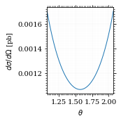

And now calculate the cross section in picobarn.

  xs_gev = total_xs_eta(η, charge, esp)
  xs_pb = gev_to_pb(xs_gev)
  tex_value(xs_pb, unit=r'\pico\barn', prefix=r'\sigma = ',
            prec=6, save=('results', 'xs.tex'))

\(\sigma = \SI{0.053793}{\pico\barn}\)

Lets plot the total xs as a function of η.

  fig, ax = set_up_plot()
  η_s = np.linspace(0, 3, 1000)
  ax.plot(η_s, gev_to_pb(total_xs_eta(η_s, charge, esp)))
  ax.set_xlabel(r'$\eta$')
  ax.set_ylabel(r'$\sigma$ [pb]')
  ax.set_xlim([0, max(η_s)])
  ax.set_ylim(0)
  save_fig(fig, 'total_xs', 'xs', size=[2.5, 2.5])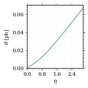

Compared to sherpa, it's pretty close.

  sherpa = np.loadtxt("../../runcards/qqgg/sherpa_xs", delimiter=",")
  tex_value(
      ,*sherpa, unit=r"\pico\barn", prefix=r"\sigma = ", prec=6, save=("results", "xs_sherpa.tex")
  )
  xs_pb - sherpa[0]

-5.112594623490896e-07

I had to set the runcard option EW_SCHEME: alpha0 to use the pure QED coupling constant.

Numerical Integration

Plot our nice distribution:

  plot_points = np.linspace(*np.arccos(interval_cosθ), 1000)
  plot_points = plot_points[plot_points > 0]

  fig, ax = set_up_plot()
  ax.plot(plot_points, gev_to_pb(diff_xs(plot_points, charge=charge, esp=esp)))
  ax.set_xlabel(r'$\theta$')
  ax.set_ylabel(r'$d\sigma/d\Omega$ [pb]')
  ax.set_xlim([plot_points.min(), plot_points.max()])
  save_fig(fig, 'diff_xs', 'xs', size=[2.5, 2.5])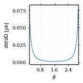

Define the integrand.

  def xs_pb_int(θ):
      return 2*np.pi*gev_to_pb(np.sin(θ)*diff_xs(θ, charge=charge, esp=esp))

  def xs_pb_int_η(η):
      return 2*np.pi*gev_to_pb(diff_xs_eta(η, charge, esp))

Plot the integrand. # TODO: remove duplication

  fig, ax = set_up_plot()
  ax.plot(plot_points, xs_pb_int(plot_points))
  ax.set_xlabel(r'$\theta$')
  ax.set_ylabel(r'$2\pi\cdot d\sigma/d\theta$ [pb]')
  ax.set_xlim([plot_points.min(), plot_points.max()])
  ax.axvline(interval[0], color='gray', linestyle='--')
  ax.axvline(interval[1], color='gray', linestyle='--', label=rf'$|\eta|={η}$')
  save_fig(fig, 'xs_integrand', 'xs', size=[3, 2.2])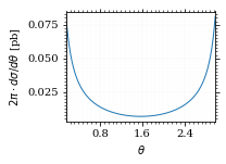

Integral over θ

Intergrate σ with the mc method.

  xs_pb_res = monte_carlo.integrate(xs_pb_int, interval, epsilon=1e-3)
  xs_pb_res

IntegrationResult(result=0.054058736201892936, sigma=0.0009406977417774582, N=2331)

We gonna export that as tex.

  tex_value(*xs_pb_res.combined_result, unit=r'\pico\barn',
            prefix=r'\sigma = ', save=('results', 'xs_mc.tex'))
  tex_value(xs_pb_res.N, prefix=r'N = ', save=('results', 'xs_mc_N.tex'))

\(N = 2331\)

Integration over η

Plot the intgrand of the pseudo rap.

  fig, ax = set_up_plot()
  points = np.linspace(-4, 4, 1000)
  ax.set_xlim([-4, 4])
  ax.plot(points, xs_pb_int_η(points))
  ax.set_xlabel(r'$\eta$')
  ax.set_ylabel(r'$2\pi\cdot d\sigma/d\eta$ [pb]')
  ax.axvline(interval_η[0], color='gray', linestyle='--')
  ax.axvline(interval_η[1], color='gray', linestyle='--', label=rf'$|\eta|={η}$')
  save_fig(fig, 'xs_integrand_eta', 'xs', size=[3, 2])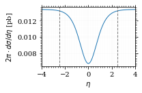

  xs_pb_η = monte_carlo.integrate(xs_pb_int_η,
                                  interval_η, epsilon=1e-3)
  xs_pb_η

IntegrationResult(result=0.053406777481589965, sigma=0.0009728516117407012, N=137)

As we see, the result is a little better if we use pseudo rapidity, because the differential cross section does not difverge anymore. But becase our η interval is covering the range where all the variance is occuring, the improvement is rather marginal.

And yet again export that as tex.

  tex_value(*xs_pb_η.combined_result, unit=r'\pico\barn', prefix=r'\sigma = ',
            save=('results', 'xs_mc_eta.tex'))
  tex_value(xs_pb_η.N, prefix=r'N = ', save=('results', 'xs_mc_eta_N.tex'))

\(N = 137\)

Using VEGAS

Now we use VEGAS on the θ parametrisation and see what happens.

  num_increments = 20
  xs_pb_vegas = monte_carlo.integrate_vegas(
      xs_pb_int,
      interval,
      num_increments=num_increments,
      alpha=2,
      increment_epsilon=0.02,
      vegas_point_density=20,
      epsilon=.001,
      acumulate=False,
  )
  xs_pb_vegas

VegasIntegrationResult(result=0.053415671595191345, sigma=0.0006275962280404523, N=280, increment_borders=array([0.16380276, 0.20536326, 0.25384714, 0.31480502, 0.39193629,
       0.48757604, 0.60550147, 0.75723929, 0.96215207, 1.23107803,
       1.56182395, 1.89731315, 2.17107801, 2.37597223, 2.52898466,
       2.64874341, 2.74453741, 2.82025926, 2.88209227, 2.93279579,
       2.9777899 ]), vegas_iterations=7)

This is pretty good, although the variance reduction may be achieved partially by accumulating the results from all runns. Here this gives us one order of magnitude more than we wanted.

And export that as tex.

  tex_value(*xs_pb_vegas.combined_result, unit=r'\pico\barn',
            prefix=r'\sigma = ', save=('results', 'xs_mc_θ_vegas.tex'))
  tex_value(xs_pb_vegas.N, prefix=r'N = ', save=('results', 'xs_mc_θ_vegas_N.tex'))
  tex_value(xs_pb_vegas.vegas_iterations, prefix=r'\times', save=('results', 'xs_mc_θ_vegas_it.tex'))
  tex_value(num_increments, prefix=r'K = ', save=('results', 'xs_mc_θ_vegas_K.tex'))

\(K = 20\)

Surprisingly, acumulation, the result ain't much different. This depends, of course, on the iteration count.

  monte_carlo.integrate_vegas(
      xs_pb_int,
      interval,
      num_increments=num_increments,
      alpha=2,
      increment_epsilon=0.02,
      vegas_point_density=20,
      epsilon=.001,
      acumulate=True,
  )

VegasIntegrationResult(result=0.053638937795766034, sigma=0.00041459931173526546, N=280, increment_borders=array([0.16380276, 0.20595251, 0.25473743, 0.31600983, 0.39036863,
       0.48642444, 0.61192596, 0.76541368, 0.96544251, 1.24106758,
       1.57551962, 1.90430764, 2.16425611, 2.36635898, 2.52157247,
       2.64333433, 2.7431946 , 2.82557121, 2.88798018, 2.93770475,
       2.9777899 ]), vegas_iterations=7)

Let's define some little helpers.

  """
  Some shorthands for common plotting tasks related to the investigation
  of monte-carlo methods in one rimension.

  Author: Valentin Boettcher <hiro at protagon.space>
  """

  import matplotlib.pyplot as plt
  import numpy as np
  from utility import *


  def plot_increments(ax, increment_borders, label=None, *args, **kwargs):
      """Plot the increment borders from a list.  The first and last one

      :param ax: the axis on which to draw
      :param list increment_borders: the borders of the increments
      :param str label: the label to apply to one of the vertical lines
      """

      ax.axvline(x=increment_borders[1], label=label, *args, **kwargs)

      for increment in increment_borders[1:-1]:
          ax.axvline(x=increment, *args, **kwargs)


  def plot_vegas_weighted_distribution(
      ax, points, dist, increment_borders, *args, **kwargs
  ):
      """Plot the distribution with VEGAS weights applied.

      :param ax: axis
      :param points: points
      :param dist: distribution
      :param increment_borders: increment borders
      """

      num_increments = increment_borders.size
      weighted_dist = dist.copy()

      for left_border, right_border in zip(increment_borders[:-1], increment_borders[1:]):
          length = right_border - left_border
          mask = (left_border <= points) & (points <= right_border)
          weighted_dist[mask] = dist[mask] * num_increments * length

      ax.plot(points, weighted_dist, *args, **kwargs)


  def plot_stratified_rho(ax, points, increment_borders, *args, **kwargs):
      """Plot the weighting distribution resulting from the increment
      borders.

      :param ax: axis
      :param points: points
      :param increment_borders: increment borders

      """

      num_increments = increment_borders.size
      ρ = np.empty_like(points)
      for left_border, right_border in zip(increment_borders[:-1], increment_borders[1:]):
          length = right_border - left_border
          mask = (left_border <= points) & (points <= right_border)
          ρ[mask] = 1 / (num_increments * length)

      ax.plot(points, ρ, *args, **kwargs)

And now we plot the integrand with the incremens.

  fig, ax = set_up_plot()
  ax.set_xlim(*interval)
  ax.set_xlabel(r"$\theta$")
  ax.set_ylabel(r"$2\pi\cdot d\sigma/d\theta$ [pb]")
  ax.set_ylim([0, 0.09])
  plot_points = np.linspace(*interval, 1000)
  ax.plot(plot_points, xs_pb_int(plot_points), label="Distribution")

  plot_increments(
      ax,
      xs_pb_vegas.increment_borders,
      label="Increment Borders",
      color="gray",
      linestyle="--",
  )

  plot_vegas_weighted_distribution(
      ax,
      plot_points,
      xs_pb_int(plot_points),
      xs_pb_vegas.increment_borders,
      label="Weighted Distribution",
  )

  ax.legend(fontsize="small", loc="lower left")
  save_fig(fig, "xs_integrand_vegas", "xs", size=[5, 3])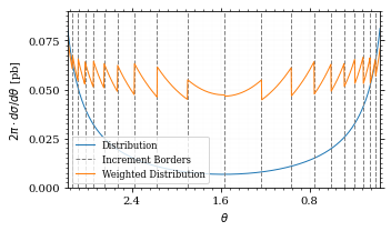

Testing the Statistics

Let's battle test the statistics.

  num_runs = 1000
  num_within = 0

  for _ in range(num_runs):
      val, err = \
          monte_carlo.integrate(xs_pb_int, interval, epsilon=1e-3).combined_result
      if abs(xs_pb - val) <= err:
          num_within += 1

  num_within/num_runs

0.688

So we see: the standard deviation is sound.

Doing the same thing with VEGAS works as well.

  num_runs = 1000
  num_within = 0
  for _ in range(num_runs):
      val, err = monte_carlo.integrate_vegas(
          xs_pb_int,
          interval,
          num_increments=num_increments,
          alpha=1,
          increment_epsilon=0.02,
          vegas_point_density=10,
          epsilon=0.1,
          acumulate=False,
      ).combined_result

      if abs(xs_pb - val) <= err:
          num_within += 1
  num_within / num_runs

/home/hiro/Documents/Projects/UNI/Bachelor/prog/python/qqgg/monte_carlo.py:451: RuntimeWarning: invalid value encountered in double_scalars
  variance = (
0.0

Sampling and Analysis

Define the sample number.

  sample_num = 1_000_000
  tex_value(
      sample_num, prefix="N = ", save=("results", "4imp-sample-size.tex"),
  )

\(N = 1000000\)

Let's define shortcuts for our distributions. The 2π are just there for formal correctnes. Factors do not influecence the outcome.

  def dist_cosθ(x):
      return gev_to_pb(diff_xs_cosθ(x, charge, esp))

  def dist_η(x):
      return gev_to_pb(diff_xs_eta(x, charge, esp))

Sampling the cosθ cross section

Now we monte-carlo sample our distribution. We observe that the efficiency his very bad!

  cosθ_sample, cosθ_efficiency = \
      monte_carlo.sample_unweighted_array(sample_num, dist_cosθ,
                                          interval_cosθ, report_efficiency=True,
                                          cache='cache/bare_cos_theta',
                                          proc='auto')
  cosθ_efficiency

0.02738751517805198

Let's save that.

  tex_value(
      cosθ_efficiency * 100,
      prefix=r"\mathfrak{e} = ",
      suffix=r"\%",
      save=("results", "naive_th_samp.tex"),
  )

\(\mathfrak{e} = 3\%\)

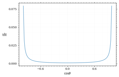
Our distribution has a lot of variance, as can be seen by plotting it.

  pts = np.linspace(*interval_cosθ, 100)
  fig, ax = set_up_plot()
  ax.plot(pts, dist_cosθ(pts))
  ax.set_xlabel(r'$\cos\theta$')
  ax.set_ylabel(r'$\frac{d\sigma}{d\Omega}$')

Text(0, 0.5, '$\\frac{d\\sigma}{d\\Omega}$')

We define a friendly and easy to integrate upper limit function.

  fig, ax = set_up_plot()
  upper_limit = dist_cosθ(interval_cosθ[0]) / interval_cosθ[0] ** 2
  upper_base = dist_cosθ(0)


  def upper(x):
      return upper_base + upper_limit * x ** 2


  def upper_int(x):
      return upper_base * x + upper_limit * x ** 3 / 3


  ax.plot(pts, upper(pts), label="upper bound")
  ax.plot(pts, dist_cosθ(pts), label=r"$f_{\cos\theta}$")

  ax.legend(fontsize='small')
  ax.set_xlabel(r"$\cos\theta$")
  ax.set_ylabel(r"$\frac{d\sigma}{d\cos\theta}$ [pb]")
  save_fig(fig, "upper_bound", "xs_sampling", size=(3, 2.5))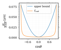

To increase our efficiency, we have to specify an upper bound. That is at least a little bit better. The numeric inversion is horribly inefficent.

  cosθ_sample_tuned, cosθ_efficiency_tuned = monte_carlo.sample_unweighted_array(
      sample_num,
      dist_cosθ,
      interval_cosθ,
      report_efficiency=True,
      proc="auto",
      cache="cache/bare_cos_theta_tuned",
      upper_bound=[upper, upper_int],
  )
  cosθ_efficiency_tuned

0.07904706665774734

<<cosθ-bare-eff>>

  tex_value(
      cosθ_efficiency_tuned * 100,
      prefix=r"\mathfrak{e} = ",
      suffix=r"\%",
      save=("results", "tuned_th_samp.tex"),
  )

\(\mathfrak{e} = 8\%\)

Nice! And now draw some histograms.

We define an auxilliary method for convenience.

  import matplotlib.gridspec as gridspec


  def draw_ratio_plot(histograms, normalize_to=1, **kwargs):
      fig, (ax_hist, ax_ratio) = set_up_plot(
          2, 1, sharex=True, gridspec_kw=dict(height_ratios=[3, 1], hspace=0), **kwargs
      )

      reference, edges = histograms[0]["hist"]
      reference_error = np.sqrt(reference)

      ref_int = hist_integral(histograms[0]["hist"])
      reference = reference / ref_int
      reference_error = reference_error / ref_int

      for histogram in histograms:
          heights, _ = (
              histogram["hist"]
              if "hist" in histogram
              else np.histogram(histogram["samples"], bins=edges)
          )
          integral = hist_integral([heights, edges])
          errors = np.sqrt(heights) / integral
          heights = heights / integral

          draw_histogram(
              ax_hist,
              [heights, edges],
              errorbars=errors,
              hist_kwargs=(
                  histogram["hist_kwargs"] if "hist_kwargs" in histogram else dict()
              ),
              errorbar_kwargs=(
                  histogram["errorbar_kwargs"]
                  if "errorbar_kwargs" in histogram
                  else dict()
              ),
              normalize_to=normalize_to,
          )

          set_up_axis(ax_ratio, pimp_top=False)
          ax_ratio.set_ylabel("ratio")
          draw_histogram(
              ax_ratio,
              [
                  np.divide(
                      heights, reference, out=np.ones_like(heights), where=reference != 0
                  ),
                  edges,
              ],
              errorbars=np.divide(
                  errors, reference, out=np.zeros_like(heights), where=reference != 0
              ),
              hist_kwargs=(
                  histogram["hist_kwargs"] if "hist_kwargs" in histogram else dict()
              ),
              errorbar_kwargs=(
                  histogram["errorbar_kwargs"]
                  if "errorbar_kwargs" in histogram
                  else dict()
              ),
              normalize_to=None,
          )

      return fig, (ax_hist, ax_ratio)


  def hist_integral(hist):
      heights, edges = hist
      return heights @ (edges[1:] - edges[:-1])


  def draw_histogram(
      ax,
      histogram,
      errorbars=True,
      hist_kwargs=dict(color="#1f77b4"),
      errorbar_kwargs=dict(),
      normalize_to=None,
  ):
      """Draws a histogram with optional errorbars using the step style.

      :param ax: axis to draw on
      :param histogram: an array of the form [heights, edges]
      :param hist_kwargs: keyword args to pass to `ax.step`
      :param errorbar_kwargs: keyword args to pass to `ax.errorbar`
      :param normalize_to: if set, the histogram will be normalized to the value
      :returns: the given axis
      """

      heights, edges = histogram
      centers = (edges[1:] + edges[:-1]) / 2
      deviations = (
          (errorbars if isinstance(errorbars, (np.ndarray, list)) else np.sqrt(heights))
          if errorbars is not False
          else None
      )

      if normalize_to is not None:
          integral = hist_integral(histogram)
          heights = heights / integral * normalize_to
          if errorbars is not False:
              deviations = deviations / integral * normalize_to

      hist_plot = ax.step(edges, [heights[0], *heights], **hist_kwargs)

      if errorbars is not False:
          if "color" not in errorbar_kwargs:
              errorbar_kwargs["color"] = hist_plot[0].get_color()

          ax.errorbar(centers, heights, deviations, linestyle="none", **errorbar_kwargs)

      ax.set_xlim(*[edges[0], edges[-1]])

      return ax


  def draw_histo_auto(points, xlabel, bins=50, range=None, rethist=False, **kwargs):
      """Creates a histogram figure from sample points, normalized to unity.

      :param points: samples
      :param xlabel: label of the x axis
      :param bins: number of bins
      :param range: the range of the values
      :param rethist: whether to return the histogram as third argument
      :returns: figure, axis
      """

      hist = np.histogram(points, bins, range=range, **kwargs)
      fig, ax = set_up_plot()
      draw_histogram(ax, hist, normalize_to=1)

      ax.set_xlabel(xlabel)
      ax.set_ylabel("Count")

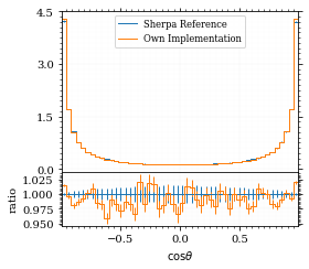
      return (fig, ax, hist) if rethist else (fig, ax)

The histogram for cosθ.

  fig, _ = draw_histo_auto(cosθ_sample, r'$\cos\theta$')
  save_fig(fig, 'histo_cos_theta', 'xs', size=(4,3))
  hist_cosθ = np.histogram(cosθ_sample, bins=50, range=interval_cosθ)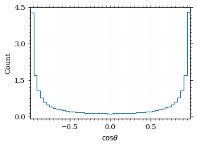

Observables

Now we define some utilities to draw real 4-momentum samples.

  @numpy_cache("momentum_cache")
  def sample_momenta(sample_num, interval, charge, esp, seed=None, **kwargs):
      """Samples `sample_num` unweighted photon 4-momenta from the
      cross-section. Superflous kwargs are passed on to
      `sample_unweighted_array`.

      :param sample_num: number of samples to take
      :param interval: cosθ interval to sample from
      :param charge: the charge of the quark
      :param esp: center of mass energy
      :param seed: the seed for the rng, optional, default is system
          time

      :returns: an array of 4 photon momenta

      :rtype: np.ndarray

      """

      cosθ_sample = monte_carlo.sample_unweighted_array(
          sample_num, lambda x: diff_xs_cosθ(x, charge, esp), interval_cosθ, **kwargs
      )

      φ_sample = np.random.uniform(0, 1, sample_num)

      def make_momentum(esp, cosθ, φ):
          sinθ = np.sqrt(1 - cosθ ** 2)
          return np.array([1, sinθ * np.cos(φ), sinθ * np.sin(φ), cosθ],) * esp / 2

      momenta = np.array(
          [make_momentum(esp, cosθ, φ) for cosθ, φ in np.array([cosθ_sample, φ_sample]).T]
      )
      return momenta

To generate histograms of other obeservables, we have to define them as functions on 4-impuleses. Using those to transform samples is analogous to transforming the distribution itself.

  """This module defines some observables on arrays of 4-pulses."""
  import numpy as np
  from utility import minkowski_product


  def p_t(p):
      """Transverse momentum

      :param p: array of 4-momenta
      """

      return np.linalg.norm(p[:, 1:3], axis=1)


  def η(p):
      """Pseudo rapidity.

      :param p: array of 4-momenta
      """

      return np.arccosh(np.linalg.norm(p[:, 1:], axis=1) / p_t(p)) * np.sign(p[:, 3])


  def inv_m(p_1, p_2):
      """Invariant mass off the final state system.

      :param p_1: array of 4-momenta, first fs particle
      :param p_2: array of 4-momenta, second fs particle
      """

      total_p = p_1 + p_2
      return np.sqrt(minkowski_product(total_p, total_p))


  def cosθ(p):
      return p[:, 3] / p[:, 0]

  def o_angle(p_1, p_2):
      eta_1 = η(p_1)
      eta_2 = η(p_2)

      return np.abs(np.tanh((eta_1 - eta_2) / 2))

  def o_angle_cs(p_1, p_2):
      eta_1 = η(p_1)
      eta_2 = η(p_2)
      pT_1 = p_t(p_1)
      pT_2 = p_t(p_2)
      total_pT = p_t(p_1 + p_2)
      m = inv_m(p_1, p_2)

      return np.abs(
          np.sinh(eta_1 - eta_2)
          ,* 2
          ,* pT_1
          ,* pT_2
          / np.sqrt(m ** 2 + total_pT ** 2)
          / m
      )

And import them.

  %aimport tangled.observables
  obs = tangled.observables

Lets try it out.

  momentum_sample = sample_momenta(
      sample_num,
      interval_cosθ,
      charge,
      esp,
      proc='auto',
      momentum_cache="cache/momenta_bare_cos_θ_1",
  )
  momentum_sample

array([[100.        ,  43.62555709,  21.21790392, -87.44490449],
       [100.        ,  41.38722348,  52.29638318, -74.51299242],
       [100.        ,  52.85217407,  65.6183037 , -53.85987297],
       ...,
       [100.        ,  49.13037192,  24.63978227, -83.54093419],
       [100.        ,  66.19768512,  12.47637819,  73.90674173],
       [100.        ,  22.11649396,  29.96005732, -92.80762717]])

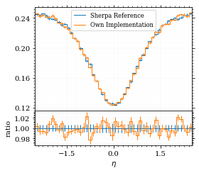
Now let's make a histogram of the η distribution.

  η_sample = obs.η(momentum_sample)
  fig, ax, hist_obs_η = draw_histo_auto(
      η_sample, r"$eta$", range=interval_η, rethist=True
  )
  save_fig(fig, "histo_eta", "xs_sampling", size=[3, 3])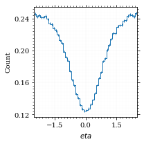

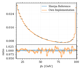
And the same for the p_t (transverse momentum) distribution.

  p_t_sample = obs.p_t(momentum_sample)
  fig, ax, hist_obs_pt = draw_histo_auto(
      p_t_sample, r"$p_T$ [GeV]", range=interval_pt, rethist=True
  )
  save_fig(fig, "histo_pt", "xs_sampling", size=[3, 3])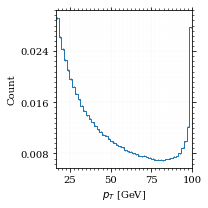

That looks somewhat fishy, but it isn't.

  fig, ax = set_up_plot()
  points = np.linspace(interval_pt[0], interval_pt[1] - .01, 1000)
  ax.plot(points, gev_to_pb(diff_xs_p_t(points, charge, esp)))
  ax.set_xlabel(r'$p_\mathrm{T}$')
  ax.set_xlim(interval_pt[0], interval_pt[1] + 1)
  ax.set_ylim([0, gev_to_pb(diff_xs_p_t(interval_pt[1] -.01, charge, esp))])
  ax.set_ylabel(r'$\frac{\mathrm{d}\sigma}{\mathrm{d}p_\mathrm{T}}$ [pb]')
  save_fig(fig, 'diff_xs_p_t', 'xs_sampling', size=[4, 2])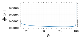

this is strongly peaked at p_t=100GeV. (The jacobian goes like 1/x there!)

Sampling the η cross section

An again we see that the efficiency is way, way! better…

  η_sample, η_efficiency = monte_carlo.sample_unweighted_array(
      sample_num,
      dist_η,
      interval_η,
      report_efficiency=True,
      proc="auto",
      cache="cache/sample_bare_eta_1",
  )
  tex_value(
      η_efficiency * 100,
      prefix=r"\mathfrak{e} = ",
      suffix=r"\%",
      save=("results", "eta_eff.tex"),
  )

\(\mathfrak{e} = 41\%\)

<<η-eff>>

Let's draw a histogram to compare with the previous results.

  η_hist = np.histogram(η_sample, bins=50)
  fig, (ax_hist, ax_ratio) = draw_ratio_plot(
      [
          dict(hist=η_hist, hist_kwargs=dict(label=r"sampled from $d\sigma / d\eta$"),),
          dict(
              hist=hist_obs_η,
              hist_kwargs=dict(
                  label=r"sampled from $d\sigma / d\cos\theta$", color="black"
              ),
          ),
      ],
  )

  ax_hist.legend(loc="upper center", fontsize="small")
  ax_ratio.set_xlabel(r"$\eta$")
  save_fig(fig, "comparison_eta", "xs_sampling", size=(4, 4))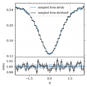

Looks good to me :).

Sampling with VEGAS

To get the increments, we have to let VEGAS loose on our distribution. We throw away the integral, but keep the increments.

  K = 10
  increments = monte_carlo.integrate_vegas(
      dist_cosθ, interval_cosθ, num_increments=K, alpha=1, increment_epsilon=0.01
  ).increment_borders
  tex_value(
      K, prefix=r"K = ", save=("results", "vegas_samp_num_increments.tex"),
  )
  increments

array([-0.9866143 , -0.96915875, -0.92958567, -0.83518973, -0.60026818,
       -0.00759974,  0.59335065,  0.83415798,  0.92874567,  0.96902194,
        0.9866143 ])

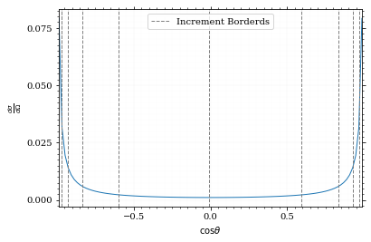
Visualizing the increment borders gives us the information we want.

  pts = np.linspace(*interval_cosθ, 100)
  fig, ax = set_up_plot()
  ax.plot(pts, dist_cosθ(pts))
  ax.set_xlabel(r'$\cos\theta$')
  ax.set_ylabel(r'$\frac{d\sigma}{d\Omega}$')
  ax.set_xlim(*interval_cosθ)
  plot_increments(ax, increments,
                  label='Increment Borderds', color='gray', linestyle='--')
  ax.legend()

<matplotlib.legend.Legend at 0x7ff0e9b4b1f0>

We can now plot the reweighted distribution to observe the variance reduction visually.

  pts = np.linspace(*interval_cosθ, 1000)
  fig, ax = set_up_plot()
  ax.plot(pts, dist_cosθ(pts), label="Distribution")
  plot_vegas_weighted_distribution(
      ax, pts, dist_cosθ(pts), increments, label="Weighted Distribution"
  )
  ax.set_xlabel(r"$\cos\theta$")
  ax.set_ylabel(r"$\frac{d\sigma}{d\cos\theta}$")
  ax.set_xlim(*interval_cosθ)
  plot_increments(
      ax, increments, label="Increment Borderds", color="gray", linestyle="--"
  )
  ax.legend(fontsize="small")
  save_fig(fig, "vegas_strat_dist", "xs_sampling", size=(3, 2.3))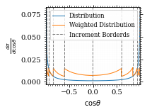

I am batman! Let's plot the weighting distribution.

  pts = np.linspace(*interval_cosθ, 1000)
  fig, ax = set_up_plot()
  plot_stratified_rho(ax, pts, increments)
  ax.set_xlabel(r"$\cos\theta$")
  ax.set_ylabel(r"$\rho")
  ax.set_xlim(*interval_cosθ)
  save_fig(fig, "vegas_rho", "xs_sampling", size=(3, 2.3))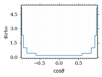

Now, draw a sample and look at the efficiency.

  cosθ_sample_strat, cosθ_efficiency_strat = monte_carlo.sample_unweighted_array(
      sample_num,
      dist_cosθ,
      increment_borders=increments,
      report_efficiency=True,
      proc="auto",
      cache="cache/sample_bare_cos_theta_vegas_1",
  )
  cosθ_efficiency_strat

0.599386385426654

  tex_value(
      cosθ_efficiency_strat * 100,
      prefix=r"\mathfrak{e} = ",
      suffix=r"\%",
      save=("results", "strat_th_samp.tex"),
  )

\(\mathfrak{e} = 60\%\)

If we compare that to /hiro/bachelor_thesis/src/commit/62a55180dda0a450297ff9d0fe0b3b5ee2c9f82b/prog/python/qqgg/cos%CE%B8-bare-eff, we can see the improvement :P. It is even better the /hiro/bachelor_thesis/src/commit/62a55180dda0a450297ff9d0fe0b3b5ee2c9f82b/prog/python/qqgg/%CE%B7-eff. The histogram looks just the same.

fig, _ = draw_histo_auto(cosθ_sample_strat, r'$\cos\theta$')
save_fig(fig, 'histo_cos_theta_strat', 'xs', size=(4,3))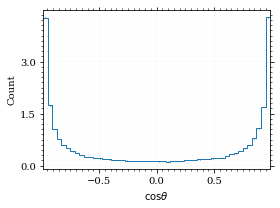

Some Histograms with Rivet

Init

  import yoda

Welcome to JupyROOT 6.20/04

Plot the Histos

  def yoda_to_numpy(histo):
      edges = histo.xEdges()
      heights = np.array([bi.numEntries() for bi in histo])

      return heights, edges


  def draw_yoda_histo_auto(h, xlabel, **kwargs):
      hist = yoda_to_numpy(h)
      fig, ax = set_up_plot()
      draw_histogram(ax, hist, errorbars=True, normalize_to=1, **kwargs)

      ax.set_xlabel(xlabel)
      return fig, ax

  yoda_file = yoda.read("../../runcards/qqgg/analysis/Analysis.yoda")
  sherpa_histos = {
      "pT": dict(reference=hist_obs_pt, label="$p_T$ [GeV]"),
      "eta": dict(reference=hist_obs_η, label=r"$\eta$"),
      "cos_theta": dict(reference=hist_cosθ, label=r"$\cos\theta$"),
  }

  for key, sherpa_hist in sherpa_histos.items():
      yoda_hist = yoda_to_numpy(yoda_file["/MC_DIPHOTON_SIMPLE/" + key])
      label = sherpa_hist["label"]
      fig, (ax_hist, ax_ratio) = draw_ratio_plot(
          [
              dict(
                  hist=yoda_hist,
                  hist_kwargs=dict(
                      label="Sherpa Reference"
                  ),
                  errorbars=True,
              ),
              dict(
                  hist=sherpa_hist["reference"],
                  hist_kwargs=dict(label="Own Implementation"),
              ),
          ],
      )
      ax_ratio.set_xlabel(label)
      ax_hist.legend(fontsize='small')
      save_fig(fig, "histo_sherpa_" + key, "xs_sampling", size=(4, 3.5))